Download
1 / 25
260 likes | 436 Vues
Interannual variability in CO2 fluxes derived from 64-region inversion of atmospheric CO2 data. Prabir K. Patra*, Shamil Maksyutov*, Misa Ishizawa*, Takakiyo Nakazawa # , Taro Takahashi $ , and Gen Inoue & *Frontier Research System for Global Change, Yokohama

E N D
Interannual variability in CO2 fluxes derived from 64-region inversion of atmospheric CO2 data Prabir K. Patra*, Shamil Maksyutov*, Misa Ishizawa*, Takakiyo Nakazawa#, Taro Takahashi$, and Gen Inoue& *Frontier Research System for Global Change, Yokohama #Graduate School of Science, Tohoku University, Sendai $Lamont-Doherty Earth Observatory, Columbia University, New York &National Institute for Environmental Studies, TSukuba Acknowledgment: TranCom-3 Developers for the TDI CODE TransCom-3 Meeting, Tsukuba, June 2004
Plan of the Talk • Basic tools • Transport model (simulation of fluxes) • Inverse model (least-squares fitting to data) • Results and Discussion • Testing of the results (networks, resolutions) • Comparisons with previous results • Climate controls on flux anomaly • Conclusions
NIES/FRSGC Tracer Transport Model: Basic Principles • The transport equations is: • where, qk is the tracer concentration with index k, S is the source function, V (s) denote the horizontal (vertical) components of winds, Fk represents the PBL flux or convective transport. We have used: • the NCEP/NCAR reanalysis data for pressure level fields • monthly PBL heights are cyclostationary (from NASA - DAO) • global distribution of yearly or monthly sources (cyclostat.)
Background CO2 fluxes: Three Types The fossil fuel emission do not have seasonality. Oceanic sources and sinks are weaker compared to the land and less heterogeneous.
Transport Model Simulations:Combined (FOS, NEP, OCN) signals of CO2 at various layers of the atmosphere (left panels) and the estimated RSDs (right panels). Patra et al., J. Geophys. Res., 2003
Estimated Flux A Priori Flux Estimated Flux Cov. A Priori Flux Cov. Inverse Model: Basic Equations The problem of surface source (S) inversion is mathematically the inversion of the forward problem: , where the G a linear operator representing atmospheric transport (no chemistry). The results are CO2 fluxes with uncertainty: Atmospheric CO2 Data
Development of 64-Regions Inverse Model Patra et al., Global Biogeochem. Cycles, submitted
Averages of CO2 Fluxes for 1990s * Spread based on sensitivity tests Patra et al., 2004a, Global Biogeochem. Cycles, submitted
Land and Ocean Flux - sensitivity Patra et al., 2004a, Global Biogeochem. Cycles, submitted
Equatorial Pacific Comparison of oceanic flux anomaly:observation and model Flux anom. (Pg-C per Year) North Pacific Patra et al., 2004a, Global Biogeochem. Cycles, Submitted
Regional Land Fluxes Patra et al., 2004b, Global Biogeochem. Cycles, Submitted
Various types of fires Indonesia ablaze, 1998. These widespread fires released massive amounts of carbon into the atmosphere
Comparisonof land flux anomalies:Observations /estimations, and Biome-BGC ecosystem model fluxes Patra et al., 2004b
Correlation Analysis CO2 Flux Anomaly With MEI ENSO Index CO2 Flux Anomaly With IOD Index
Flux Anom./PC vs. Met./Clim. Index Region/PC ENSO IOD Rain* Temp. Temp. N. A. -0.41 -0.34 -0.39 0.30 Trop. S. A. 0.49 0.51 -0.51 0.66 Temp. Asia -0.19 0.17 0.11 -0.15 Trop. Africa 0.73 0.44 0.37 0.47 South Africa 0.66 0.54 0.00 0.07 Trop. Asia 0.53 0.46 -0.68 0.55 Australia 0.36 0.35 -0.19 0.18 PC - 1 0.91 0.76 PC - 2 -0.46 -0.22 PC - 3 0.25 -0.13 * CO2 flux anomaly lags 3-month the rainfall anomaly. In Tropics: CO2 flux & Temp: +ve CO2 flux & Rain : -ve
In search of simple empirical relations Green diamond: van der Werf et al. Vertical bar: Kasischke and Bruhwiler
Conclusions • We have derived CO2 fluxes from 42 land and 22 ocean regions. • The inverse method fairly successfully captures the flux variability due to climate variation. • The highest influence of weather/climate is observed over the tropical lands. • Major modes of CO2 flux variability are connected to ENSO/IOD, Biomass burning (indirect climate forcing?). • Interannual variability in MLO CO2 growth rates are mostly of natural origin (as in Keeling et al., 1995)