Download
1 / 59
590 likes | 816 Vues
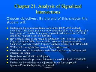
Chapter 21. Analysis of Signalized Intersections. Chapter objectives: By the end of this chapter the student will:.

E N D
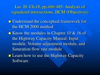
Chapter 21. Analysis of Signalized Intersections Chapter objectives: By the end of this chapter the student will: • Understand the conceptual framework for the HCM 2000 method, including Critical lane group, v/s ratio, saturation flow rate, capacity of a lane group, v/c ratio for lane group, approach and intersection v/c, LOS, and effective green times and lost time • Have general ideas of the modules in Chapter 10 & 16 of the Highway Capacity Manual 2000: Input module, Volume adjustment module, Saturation flow rate module, Capacity analysis module, and LOS module • Will be able to explain how Arrival Type is determined • Know how to enter input data into the Highway Capacity Software and interpret the output • Know how to deal with initial queues • Understand how the permitted left turns are modeled by the 2000 HCM • Understand how the left-turn adjustment factor for compound (protected/permitted) phasing is modeled. Chapter 21
21.1 Introduction • Highway Capacity Manual 2000, Chapter 10 & 16, Consisting primarily of deterministic analytic algorithms developed from theoretical considerations and/or empirical data and regression analysis and its companion Highway Capacity Software (HCS) • SOAP (“simulation” and optimization) • Synchro Studio 7.0 (“simulation” and optimization, HCS analysis) • Transyt 7F (“simulation” and optimization, network of signalized intersections) • PASSER II (Signalized arterial analysis) • HCS Cinema & SigCinema (HCS + simulation based on NETSIM) • SimTraffic (simulation) • CORSIM (simulation) Chapter 21
21.1 Conceptual framework for HCM 2000 Five fundamental concepts of the HCM 2000: • The critical lane group concept • The v/s ratio as a measure of demand • Capacity and saturation flow rate concepts • Level-of-service criteria and concepts • Effective green time and lost-time concepts Chapter 21
21.1 Conceptual framework for HCM 2000 21.2.1. Critical lane group concept Critical lane analysis (Section 17.3) vs. Critical lane group analysis v c v c Critical lane analysis compares actual flow (v) with the saturation flow rate (s) and capacity (c) in a single lane. Critical lane group analysis compares actual flow (v) with the saturation flow rate (s) and capacity (c) in a group of lanes operating in equilibrium. In either case, the ratio of v to c is the same (when traffic is evenly distributed among the lanes in a lane group). This applies to shared lanes, also. Exclusive right- or left-turn lanes must be separately analyzed because they are separate lane groups. Lane utilization is considered in computing saturation flow rate. Chapter 21
21.2.2 The v/s ratio as a measure of demand & 21.2.3 Capacity and saturation flow rate concepts * The simple method in Chapter 18 (as a comparison – Vc is adjusted by converting into tvu (through vehicle unit) & saturation flow is given): * The HCM 2000 model adjusts saturation flow rate and considers 11 specific conditions affecting intersection operations: (1) Lane width, (2) Heavy vehicle presence, (3) Grade, (4) Parking conditions, (5) Local bus blockage, (6) Location within the urban area, (7) Lane utilization, (8) Left turns, (9) Right turns, (10) Pedestrian-bike adjustment for LT movements, and (11) Pedestrian-bike adjustment for RT movements. All adjustments are used to modify an ideal saturation flow rate to one that represents prevailing conditions for the lane group. (7), (10), and (11) are new additions to the 1994 model. We may not be able to compare directly lane groups because their conditions are different. So HCM use the flow ratio, v/s. This process is called “normalization.” Chapter 21
Capacity • In the simple timing method in Chapter 18, the capacity of the intersection as a whole was considered. • HCM 2000 as well as 1994 HCM gives the capacity of each lane group. • Demand does not necessarily peak at all approaches at the same time. • Capacity may change for each approach during the day. (like the effect of curb side parking, bus blocking, etc.) • Capacity is provided to movements to satisfy movement demands. (Note: the critical capacity ratio v/c (for the intersection as a whole) is still calculated in HCM 2000) Chapter 21
For each critical lane group analysis calculate: 1. Saturation flow rate Saturation flow rate for a lane group Ideal saturation flow rate, 1900 pcphgpl 2. Capacity of a lane group Chapter 21
v/c ratios. “degree of saturation” • Three issues: • Capacity is practically always estimated (because it is difficult to measure.) • In existing cases demand is often measured by “departure flows” although it should be “arrival flows.” • For future cases, predicted arrival volumes are given (by a planning model) instead of actually counted volumes. Case 1 & 2: v/c > 1.0 resulted in a HCM analysis for an existing signalized intersection. If demand is measured by a departure flow (assuming it was correct), this cannot be accepted because max value v/c = 1.0. If arrival flows are measured, v/c > 1.0 may occur – this becomes obvious because queue forms). Capacity must have been underestimated if queue is not formed despite the fact v/c > 1.0 results because HCM models are based on national average values. Chapter 21
Case 3: v/c > 1.0 resulted in an analysis for a planned signalized intersection. In a planning case, both demand and capacity are estimates. But, it may indicate that the forecast demand flow exceeds the estimated capacity of the lane group, and a problem will likely exist. Demand is an arrival flow for a predicted case because those values come from a planning model. Computation of a v/c ratio for a given lane group (this model does not change: Flow ratio/Green ratio Chapter 21
Computation of a v/c ratio for an intersection as a whole: The critical v/c ratio for the intersection defined as the sum of the critical lane group flows divided by the sum of the lane group capacities available to serve them (compare this one with the Simple Method in Ch 17). If the Xc > 1.0, then the physical design, phase plan, and cycle length specified do not provide sufficient capacity for the anticipated or existing critical lane group flows. Do something to increase capacity: (1) longer cycle lengths, (2) better phase plans, and (3) add critical lane group or groups (meaning change approach layouts) Chapter 21
Computation of a v/c ratio for an intersection as a whole (Additional comments): • If the critical v/c ratio is less than 1.00, the cycle length, phase plan, and physical design provided are sufficient to handle the demand and flows specified. • But, having a critical v/c ratio under 1.00 does not assure that every critical lane group has v/c ratios under 1.00. When the critical v/c ratio is less than 1.00, but one or more lane groups have v/c rations greater than 1.00, the green time has been misallocated. Chapter 21
21.2.4 Level of service concepts and criteria • All the HCM delay models assume random arrivals. Hence, the delay model produce delays for approaches with random arrivals. Urban signals are coordinated; hence, many do not have random arrivals. This is corrected by the “quality of progression” factor called “Arrival Type” factor. See Table 21.5 and 21.6. There are 6 arrival types: 1 = poor coordination, 6 = exceptional coordination. • For uninterrupted facilities, like freeways, v/c has a direct connection with the performance of the facility. So, if v/c = 1.0, the facility is at the capacity. • For signalized intersections (interrupted facilities), this is not necessarily true – especially when delay is used as the MOE. • You may get LOS=F even if v/c is well below 1.0. For instance LT vehicles may have a long stopped delay even if its v/c is low. • HCM 1994 delay model focuses on the first 15-min interval. So, even if it is over-saturated (v/c > 1.0), we get a relatively smaller delay. HCM 2000 has 3 study approaches: Single analysis period for 15 min and 1 hour, and multiple 15-min analysis periods (See Exhibit 16-6 in HCM 2000.) Chapter 21
The 2000 HCM uses “average control delay” consisting of three terms d1 = uniform control delay. You must divide d1 obtained by HCM 2000 by 1.3 to compare with d1 by HCM 1994 (stopped delay). d2 = adjustment for randomness d3 = adjustment for initial queue (left over vehicles caused by oversaturation in the previous cycle) The delay models are discussed in section 21.3.7. Chapter 21
A B C D 21.2.5 Effective green times and lost times • Actual signal indications • Actual use of green and yellow; e is extended green, i.e. part of the yellow used as green • Lost times l1 and l2 are added and placed at the beginning of the green for modeling purposes • Effective green and effective red l1 = 2 sec/phase e = 2 sec/phase Default by HCM2000 Chapter 21
Effective green times and the application of the lost times: • HCM delay models use “effective green time” and “effective red time.” • HCM 2000 models assume that all lost times happen at the beginning of the phase. gi ri tL Watch out where tL takes place, especially when an overlap phase exists. That’s where you must add y and ar in the phase section of the HCS+ input module. Chapter 21
21.3 The Basic Model 21.3.1 Model structure The HCM 2000 signalized intersection analysis consists of 5 modules. Compare them with the input/output sections of HCS+. Chapter 21
21.3.2 Analysis time periods • The peak 15 minutes within the analysis hour (no over-saturation exists, no v/c > 1.0. Use PHF.) • The full 60-min analysis hour (OK, but masks the peak.) • Sequential 15-min periods for an analysis period of one hour or greater (Most comprehensive. PHF = 1.0 is used. Chapter 21
21.3.3 Input Module Input Module: Many parameters are considered. See Exhibit 16-3 (Table 21-3 in the text). Geometric, traffic, and signalization conditions are considered Some of them are self-explanatory. • Area type: CBD intersections have lower saturation flow rates (in general). Saturation flow rates for CBD is about 10% less than for non-CBD. • Parking conditions and parking activity: Parking activity within 250 ft of the stop line is considered. Parking activities interfere traffic flow • Conflicting pedestrian flow (for RT vehicles): Pedestrian flow between 1700 to 2100 ped/hr completely blocks right-turn vehicles. HCM 2000 considers bicycles as well. Also, check pedestrian min green times • Local bus volume: Buses must stop to be considered in this parameter. If they pass through the intersection, not stopping for passengers, they are considered as heavy vehicles. • Arrival type: The single most important factor influencing delay predictions. Chapter 21
More discussion on Arrival type (Exhibit 16-4, p.595 text): Chapter 21
A. Input Module (cont) More discussion on Arrival type: Need to compute a platoon ratio: P = Proportion of vehicles arriving on green. Rp = 1.00, when the proportion of vehicles arriving on green is equal to the g/C ratio. (Same as Exhibit 16-11 of HCM 2000.) These Rp values are used to determine PF values. See Table 21-5 on page 596. See Table 21.8 for PF values. Chapter 21
21.3.4 Volume Adjustment Module 1. Conversion of hourly demand volumes to peak 15-min flow rates 2. Establish lane groups for analysis Defacto LT lane: A shared TH-LT lane is functioning like a left-turn lane because there are so many LT vehicles. There is no way to know it from the beginning. So start the HCM procedure that there is no de-facto LT lane. In the procedure the proportion of LT vehicles in the left lane (PL) is estimated. If PL = 1.00, the lane becomes a Defacto LT lane. And you start the computation from the start! See Eq. 21-52 in page 633 for PL’s definition. 3. Determination of total lane group demand flow rates, vgi Chapter 21
21.3.5 Saturation Flow Rate Module The saturation flow rate module is the most important part of HCM2000. The prevailing total saturation flow rate for each lane group is estimated. • This is a HCM2000 saturation flow model. Compare with the one in the text which comes from HCM1994. First 7 are easy; the last two factors are really involved. Chapter 21
Right-turn adjustment factor, fRT (modified): The pedestrian effect term was removed and two new factors for pedestrian-bicycle blockage effect were created: fRpb and fLpb) Chapter 21
Left-turn adjustment factor, fLT Exclusive LT lane with protected LT phasing Exclusive LT lane with permitted LT phasing Exclusive LT lane with compound LT phasing Shared LT lane with protected phasing Shared LT lane with permitted phasing Shared LT lane with compound phasing Case 4 is rare because it may waste green time. Case 6 may waste green time, also. Section 21.5 discusses permitted LT and compound phasing cases. Appendix C of the 2000 HCM discusses the models. Chapter 21
Adjustment factors for LT (fLT) (Slower turning speeds are the major factor for this case.) (When PLT = 1, a defacto LT lane, fLT is about 0.95.) Logical choices Chapter 21
21.3.6 Capacity analysis module HCM-way of determining lane groups and the sum of critical lane group v/s ratios • In a simple signal timing method, critical lane groups were determined by comparing adjusted per lane flows in each lane group using a ring diagram. Chapter 17.3. • In the 2000 HCM, per-lane flows cannot be compared because we have lane group flows. So, we use v/s ratios to determine critical lane groups. • Once the v/s is computed (the outcomes of Module 2 and 3 of the 2000 HCM), v/s is used to determine critical lane groups and a ring diagram is again used to determine them. Chapter 21
The v/s ratio for each lane group is computed • Relative v/s ratios are used to identify the critical lane groups in the phase plan; the sum of critical lane group v/s ratios is computed • Lane group capacities are computed • Lane group v/c ratios are computed • The critical v/c ratio for the intersection is computed. Eq 21-2 Eq 21-3 Eq 21-5 Chapter 21
Modifying signal timing based on v/s ratios • After v/s ratios are computed, we may need to make adjustments – either reallocation of green time, modifying cycle length, or modifying the intersection layout. For the first two cases, v/s ratios can be used to reduce the amount of trial-and-error computations. First, we solve Xc for C: When Xc = 1.0, it is like C equation for simple signal timing (eq. 17-13). • Suppose sum(v/s) = 0.9, and we desire to achieve Xc = 0.95. What would be the cycle length to serve this (assume max C = 90 sec)? Xc = 0.95 cannot be achieved in this case. C = 171 sec is too long. Chapter 21
Modifying signal timing based on v/s ratios (cont) • C needs to be contained within the common cycle lengths (171 sec in the previous example is too long). Typically C = 120 sec is the maximum cycle length accepted. Hence, Where, Σgi = C – L. With sum(v/s) = 0.90 and C = 120 sec, Xc = 0.973 is the minimum that can be achieved. Once C is determined, we can compute new effective greens,then new actual greens for the next trial-and-error analysis. Chapter 21
21.3.7 LOS module • This is the last step—estimating average individual stopped delays for each lane group. 1. Delay models for standard cases (for permitted or protected or compound phasing phasing from a shared lane group): (eq. 21-30) (eq. 21-31) (eq. 21-32) (eq. 21-35) Chapter 21
Arrival Type determination review More discussion on Arrival type: Need to compute a platoon ratio: P = Proportion of vehicles arriving on green. Rp = 1.00, when the proportion of vehicles arriving on green is equal to the g/C ratio. (Same as Exhibit 16-11) These Rp values are used to determine PF values. See Table 21.8 on page 608. Chapter 21
Progression adjustment factor (PF) Chapter 21
Delay adjustment (k) for controller type (actuated or non-actuated) for the incremental delay term, d2 Chapter 21
Upstream Filtering or Metering Adjustment Factor, I • An I-value of 1.0 is used for an isolated intersection (i.e., one that is 1 mile or more from the nearest upstream signalized intersection). This value is based on a random number of vehicles arriving per cycle so that the variance in arrival equals the mean.) • An I-value of less than 1.0 is used for non-isolated intersections. This reflects the way that upstream signals decrease the variance in the number of arrivals per cycle at the subject intersection. As a result, the amount of delay due to random arrivals is reduced. Chapter 21
Initial queue delay HCM 2000 cases: • Case 1: No initial queue, X≤1.00 • Case 2: No initial queue, X>1.00 • Case 3: Initial queue, X<1.00, no residual queue at end of analysis period • Case 4: Initial queue, X<1.00, residual queue exists at end of analysis period but is less than the size of the initial queue • Case 5: Initial queue, X≥1.00, residual queue exists at end of analysis period and is the same or larger than the size of the initial queue Chapter 21
Determining whether Case 3, 4, or 5 exists. • Total demand (v/hr) during the analysis period T (hr) with Qb initial queue at the beginning of analysis period T: • Ndem = Qb + vT • Capacity (v/hr) during analysis period T: • Ncap = cT • Assuming that an initial queue exists (i.e., Qb > 0): • Case 3 exists when Ndem≤ Ncap • Case 4 exists when Ndem > Ncap and v < c • Case 5 exists when Ndem > Ncapand v ≥ c • For Cases 1 and 2, there is no delay due to the existence of an initial queue, and d3 is zero. • For Cases 3, 4, and 5, use 1800 =3600/2: used to convert the unit of C (veh/hr) to (veh/sec) because delay is expressed in sec/veh. ½ is a shape factor for a triangle and a trapezoid showing the effect of delays by the initial queue. Chapter 21
Determining whether Case 3, 4, or 5 exists. t = duration of oversaturation within T, h (Unused capacity is used to clear Qb) u = delay parameter Hence the total delay for these cases are: (Note that PF is not multiplied to d1 like equation 21-3.) X = 1 for ds and X = actual for du. Chapter 21
The size of the queue at the beginning of any time period (i+1) Aggregating delay: Chapter 21
21.3.8 Interpreting the results of signalized intersection analysis • v/c ratio for every lane group • Critical v/c ratio (Xc) for the intersection as a whole • Delays and levels of service for each lane group • Delays and levels of service for each approach • Delays and levels of service for the overall intersection • The following scenarios are possible: • Scenario 1: Xc ≤ 1.00, all Xi ≤ 1.00. No capacity deficiency • Scenario 2: Xc ≤ 1.00, some Xi > 1.00. As long as Xc ≤ 1.00, the current conditions can handle; reallocate green times • Scenario 3: Xc > 1.00, some or all Xi > 1.00. Need to change timing and if necessary physical layout changes Chapter 21
21.4 Some “Simple” Sample Problems • Problems 1, 2, and 3. See the discussions in the text Chapter 21
21.5 Complexities with LTs • Left-turn adjustment factor, fLT, for permitted left turns • Analysis of compound LT phasing • Using analysis parameters to adjust signal timing (review it by yourself) • Analysis of actuated signals (review it by yourself) – With HCS 2000 you may use the SOAP’s actuated signal estimator. Chapter 21
21.5.1 LT Adjustment factor for permitted LTs Interaction between LT vehicles and opposing vehicles • No gaps are available for LTs when the standing queue is released right after the signal turns green. • If a LT vehicle arrives during this time, it must wait, blocking the left-most lane, until the opposing queue has cleared. • After the opposing queue has cleared the intersection, LTs may be made through gaps in the unsaturated opposing flow. • LTs have no impact on the subject approach until the first LT vehicle arrives (for a shared LT lane). X gq = avg. amount of green time required for the opposing standing queue to clear the intersection, sec. gf = avg. amount of green time before the arrival of the 1st LT vehicle, sec (gf = 0.0 sec for an exclusive LT lane) gu = avg. amount of green time after the arrival of the 1st LT vehicle that is not blocked by the clearance of the opposing standing queue, sec
Modeling permitted left-turns (cont) Opposing queued vehicles clearing Green not blocked by the opposing clearing queue, usable by LT vehicles The first LT vehicle must wait. Opp. Queued vehicle clearing Green not blocked by the opposing clearing queue, usable by LT vehicles First LT veh has not arrived yet Chapter 21
Modeling permitted left-turns (cont) Basic structure of the permitted LT model (general concept) The model must consider: • How LT vehicles are affected during various portions of the green phase. • How those LT vehicles affect the general operation of the lane group. • 1st, determine a LT adjustment factor, fm, that applies only to the left-most lane from which LTs are made. • This factor, fm, is later combined to find the total impact on the lane group. Where there is only one (or double) exclusive left-turn lane in the lane group, fm = fLT. (eq. C16-2 HCM2000 and 21-42 in the text) 1.00 >= F1 >= 0.0 F2 = 0 when opposing approach is multilane. Why? Chapter 21
Basic structure of the permitted LT model (cont): multilane This equation allows for a value of fm of zero. This happens when g = gq (gu = g – gq=0); the opposing standing queue blocks the intersection to LT vehicles for the entire green interval. But, there are always SNEAKERS during Yellow or AR intervals; hence the minimum value needs to be established. But the minimum is: Observations show at least one vehicle can turn during the clearance interval and may be two if the second vehicle is a LT vehicle. 2 = 2 second headway, 1 = minimum 1 LT sneaker, and PL is the proportion (probability, that is) of LT vehicles in the left lane. When a single (or double) exclusive-permitted LT lane is involved fLT = fm. If there are more lanes (meaning through lanes) in the lane group, meaning a shared lane exists, the effective LT adjustment for other lanes is 0.91. N is the number of lanes in the lane group; -1 is the left-most lane. The lane group includes a shared LT lane Chapter 21
Basic structure of the permitted LT model (cont) F1 values are computed as follows: For EL1, see Exhibit C16-3 in HCM 2000. Table 21.18. Everything discussed up to here applies to all types of lane groups that are opposed by multilane approaches. Now we consider single-lane opposing approaches. Chapter 21
Basic structure of the permitted LT model (cont): single-lane opposing approaches When the opposing flow is in a single-lane approach, a LT vehicle on that approach creates a gap in the opposing flow through which a subject LT vehicle may move. We need to consider this available gap (2nd term below), which does not exist if there are multiple lanes in the opposing approach. (eq. C16-8 and 21-44 in the text) Proportion of through and RT vehicles in the opposing single-lane approach, decimal. Proportion of LT vehicles in the opposing single-lane approach, decimal n = No. of opposing vehicles in the period gq – gf, about (gq – gf)/2. n can be zero. 2 is 2 sec/veh headway and n is for joint probability. The numerator is the probability that one or more vehicles are LT vehicles. Chapter 21
Now we need to estimate gf These models are empirical models. • When the subject approach has more than one lane (for shared permitted LT lanes): (eq. C16-5 & 21-47) • When the subject approach has one lane (shared single-lane groups): (eq. C16-7 & 21-47) Where, G = actual green time for lane group, sec LTC = LTs per cycle, [(vLT/3600) x C] vLT = LT flow rate in subject lane group, vph tL = total lost time per phase, sec gf = 0 for exclusive LT lanes. A LT veh exists from the beginning of green Chapter 21