Download
1 / 57
640 likes | 1.59k Vues
Chapter 24. Analysis of Signalized Intersections. Chapter objectives: By the end of this chapter the student will:.

E N D
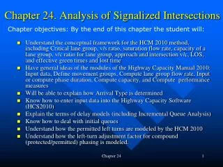
Chapter 24. Analysis of Signalized Intersections Chapter objectives: By the end of this chapter the student will: • Understand the conceptual framework for the HCM 2010 method, including Critical lane group, v/s ratio, saturation flow rate, capacity of a lane group, v/c ratio for lane group, approach and intersection v/c, LOS, and effective green times and lost time • Have general ideas of the modules of the Highway Capacity Manual 2010: Input data, Define movement groups, Compute lane group flow rate, Input or compute phase duration, Compute capacity, and Compute performance measures • Will be able to explain how Arrival Type is determined • Know how to enter input data into the Highway Capacity Software (HCS2010) • Explain the terms of delay models (including Incremental Queue Analysis) • Know how to deal with initial queues • Understand how the permitted left turns are modeled by the HCM 2010 • Understand how the left-turn adjustment factor for compound (protected/permitted) phasing is modeled. Chapter 24
24.1 Introduction • What’s new in HCM 2010 as compared with HCM 2000 • The model has been set up to handle actuated signal analysis directly. • The estimation of delay is now partially modeled using Incremental Queue Analysis (IQA). IQA allows a more detailed analysis of arriving and departing vehicle distributions. • The definition of lane groups has been altered. Lane groups are identified and separately analyzed as part of the methodology. “This text focuses on the analysis of pretimed signals because it is more straight forward to present basic modeling theory for fixed time signals.” Chapter 24
HCM 2010 Analysis Steps Chapter 24
24.1 Conceptual framework for HCM 2010 Five fundamental concepts of the HCM 2010: • The critical lane group concept • The v/s ratio as a measure of demand • Capacity and saturation flow rate concepts • Level-of-service (LOS) criteria and concepts • Effective green time and lost-time concepts Chapter 24
24.2.1 The Critical-Lane Group Concept Critical lane analysis (Section 17.3) vs. Critical lane group analysis Critical lane analysis compares actual flow (v) with the saturation flow rate (s) and capacity (c) in a single lane. Critical lane group analysis compares actual flow (v) with the saturation flow rate (s) and capacity (c) in a group of lanes operating in equilibrium. In either case, the ratio of v to c is the same (when traffic is evenly distributed among the lanes in a lane group). This applies to shared lanes, also. Exclusive right- or left-turn lanes must be separately analyzed because they are separate lane groups. Lane utilization is considered in computing saturation flow rate. Chapter 24
24.2.2 The v/s ratio as a measure of demand & 24.2.3 Capacity and saturation flow rate concepts * The simple method in Chapter 21 (as a comparison – Vc is adjusted by converting into tvu (through vehicle unit) & saturation flow is given): * In the HCM model, demand flow rates are not converted to tvu. It uses veh/hr (though adjusted for PHF). A key part of the HCM 2010 model is a methodology for estimating the saturation flow rate of any lane group based on known prevailing traffic parameters. We may not be able to compare directly lane groups because their conditions are different. So HCM use the flow ratio, v/s, a dimensionless value for comparison purposes. This process is called “normalization.” Chapter 24
24.2.3 Capacity (continued) • In the simple timing method in Chapter 21, the capacity of the intersection as a whole was considered. • HCM 2010 as well as HCM 2000 gives the capacity of each lane group. • Demand does not necessarily peak at all approaches at the same time. • Capacity may change for each approach during the day. (like the effect of curb side parking, bus blocking, etc.) • Capacity is provided to movements to satisfy movement demands. (Note: the critical capacity ratio v/c (for the intersection as a whole) is still calculated in HCM 2010 just like HCM 2000). Chapter 24
The v/c ratio “degree of saturation” • Three issues: • Capacity is practically always estimated (because it is difficult to measure.) • In existing cases demand is often measured by “departure flows” although it should be “arrival flows.” • For future cases, predicted arrival volumes are given (by a planning model) instead of actually counted volumes. Case 1 & 2: v/c > 1.0 resulted in a HCM analysis for an existing signalized intersection. If demand is measured by a departure flow (assuming it was correct), this cannot be accepted because max value v/c = 1.0. If arrival flows are measured, v/c > 1.0 may occur – this becomes obvious because queue forms). Capacity must have been underestimated if queue is not formed despite the fact v/c > 1.0 results. Capacity underestimation is possible because HCM models are national average models. Chapter 24
Case 3: v/c > 1.0 resulted in an analysis for a planned signalized intersection. In a planning case, both demand and capacity are estimates. But, it may indicate that the forecast demand flow exceeds the estimated capacity of the lane group, and a problem will likely occur. Demand is an arrival flow for a predicted case because those values come from a planning model. Computation of a v/c ratio (degree of saturation) for a given lane group (this model does not change among different HCM versions: Flow ratio/Green ratio Chapter 24
Computation of a v/c ratio for an intersection as a whole (p.576): The critical v/c ratio for the intersection defined as the sum of the critical lane group flows divided by the sum of the lane group capacities available to serve them (compare this one with the Simple Method in Ch 20). If the Xc > 1.0, then the physical design, phase plan, and cycle length specified do not provide sufficient capacity for the anticipated or existing critical lane group flows. Do something to increase capacity: (1) longer cycle lengths (less number of cycles, less lost time), (2) better phase plans (improved LT treatment), and (3) add critical lane group or groups (meaning change approach layouts increase capacity) Chapter 24
Computation of a v/c ratio for an intersection as a whole (Additional comments): • If the critical v/c ratio is less than 1.00, the cycle length, phase plan, and physical design provided are sufficient to handle the demand and flows specified. • But, having a critical v/c ratio under 1.00 does not assure that every critical lane group has v/c ratios under 1.00. When the critical v/c ratio is less than 1.00, but one or more lane groups have v/c rations greater than 1.00, the green time has been misallocated. Chapter 24
24.2.4 Level of service concepts and criteria • All the HCM delay models assume random arrivals. Hence, the delay model produce delays for approaches with random arrivals. Urban signals are coordinated; hence, many do not have random arrivals. This is corrected by the “quality of progression” factor called “Arrival Type” factor. See Table 24.3 and 24.4. There are 6 arrival types: 1 = poor coordination, 6 = exceptionally good coordination. • For uninterrupted facilities, like freeways, v/c has a direct connection with the performance of the facility. So, if v/c = 1.0, the facility is at the capacity. • For signalized intersections (interrupted facilities), this is not necessarily true – especially when delay is used as the MOE. • You may get LOS=F even if v/c is well below 1.0. For instance LT vehicles may have a long stopped delay even if its v/c is low. • HCM 1994 delay model focuses on the first 15-min interval. So, even if it is over-saturated (v/c > 1.0), we get a relatively smaller delay. HCM 2010 has 3 study approaches: Single analysis period for 15 min and 1 hour, and multiple 15-min analysis periods. Chapter 24
The 2010 HCM uses “total control delay” consisting of three terms Total control delay per vehicle = time in queue delay + acceleration-deceleration delay New to HCM 2010: Any lane group operating at a v/c ratio greater than 1.00 is also labeled as LOS F. Because delay is difficult to measure in the field and because it cannot be measured for future situations, delay is estimated using analytic models. The delay models are discussed in section 24.3.7. Chapter 24
A B C D 24.2.5 Effective green times and lost times • Actual signal indications • Actual use of green and yellow; e is extended green, i.e. part of the yellow used as green • Lost times l1 and l2 are added and placed at the beginning of the green for modeling purposes • Effective green and effective red l1 = 2 sec/phase e = 2 sec/phase Default by HCM2010 Chapter 24
Effective green times and the application of the lost times: • HCM delay models use “effective green time” and “effective red time.” • HCM 2010 models assume that all lost times happen at the beginning of the phase. Watch out where tL takes place, especially when an overlap phase exists. That’s where you must add y and ar in the phase section of the HCS input module. Chapter 24
24.3 The Basic Model 24.3.1 Model structure The HCM 2010 signalized intersection analysis consistsof 6 modules. Chapter 24
24.3.2 Analysis time periods • The peak 15 minutes within the analysis hour (no over-saturation exists, no v/c > 1.0. Use PHF.) • The full 60-min analysis hour (OK, but masks the peak.) • Sequential 15-min periods for an analysis period of one hour or greater (Most comprehensive. PHF = 1.0 is used. Chapter 24
24.3.3 Input Input Module: Many parameters are considered. See Table 24-2 in the text). Geometric, traffic, and signalization conditions are considered Some of them are self-explanatory. See pages 582 – 585 for details and default values. • Area type: CBD intersections have lower saturation flow rates (in general). Saturation flow rates for CBD is about 10% less than for non-CBD. • Parking conditions and parking activity: Parking activity within 250 ft of the stop line is considered. Parking activities interfere traffic flow • Conflicting pedestrian flow (for RT vehicles): Pedestrian flow between 1700 to 2100 ped/hr completely blocks right-turn vehicles. HCM 2010 considers bicycles as well. Also, check pedestrian min green times • Local bus volume: Buses must stop to be considered in this parameter. If they pass through the intersection, not stopping for passengers, they are considered as heavy vehicles. • Arrival type: The single most important factor influencing delay predictions. Chapter 24
More discussion on Arrival type (Table 24.3, p.583 text): P = Proportion of vehicles arriving on green. Chapter 24
More discussion on Arrival type: Need to compute a platoon ratio, Rp: P = Proportion of vehicles arriving on green. Rp = 1.00, when the proportion of vehicles arriving on green is equal to the g/C ratio. Table 24.4 (They accidentally (?) forgot two columns for platoon ratio. Chapter 24
24.3.4 Movement Groups, Lane Groups, and Demand Volume Adjustment 1. Conversion of hourly demand volumes to peak 15-min flow rates needs to be done first. 2. Establish analysis lane groups (6 types) These two rules are new in HCM2010. Chapter 24 3. Determination of total lane group demand flow rates, vgi
Figure 24.5 Common Movement and Lange Groups on a Signalized Intersection Approach New in HCM2010 Chapter 24
24.3.5 Estimating the Saturation Flow Rate for Each Lane Group The saturation flow rate module is the most important part of HCM2010. The prevailing total saturation flow rate for each lane group is estimated. • Adjustment for Lane Width: • fw = 0.96 Lane width < 10ft • fw = 1.00 10 ft ≤ Lane width ≤ 12.9 ft • fw = 1.04 Lane width ≥ 12.9 ft Chapter 24
Adjustment for Heavy Vehicles: Adjustment for Grade: EHV = 2.00 Adjustment for Parking Conditions: • Limitations: • 0 ≤ Nm ≤ 180; if Nm > 180, use 180 mvts/h • fp(min) = 0.05 • fp(no parking) = 1.00 Chapter 24
Adjustment for Local Bus Blockage: • Limitations: • 0 ≤ NB ≤ 250; if NB > 250, use 250 b/h • fbb(min) = 0.05 • Adjustment for Type of Area: • CBD location: fa = 0.90 • Other location: fa = 1.00 Adjustment for Lane Utilization: See Table 24.7 for default values (next page). Chapter 24
Adjustment for Lane Utilization (continued): Chapter 24
Adjustment for Right Turns: • From an exclusive RT lane (fRT = 0.85) • From a shared lane • From a single-lane approach Adjustment for Left Turns (discussed in section 24.5 of the text): • Case 1: Exclusive LT lane with protected phasing (fLT = 0.95) • Case 2: Exclusive LT lane with permitted phasing • Case 3: Exclusive LT lane with compound phasing • Case 4: Shared lane with protected phasing • Case 5: Shared lane with permitted phasing • Case 6: Shared lane with compound phasing Chapter 24
Adjustment for Pedestrian and Bicycle Interference with Turning Vehicles (There are seven steps; see pages 589-591): Chapter 24
Pedestrian and Bike Interference Adjustment (continued): gped = walk + clearance interval • 2,000 = 3,600/1.8 sec a ped occupies the ped conflict area. • 10,000 = 3,600/0.36 sec a ped occupies the ped conflict area walking parallel. 0.4 = 40% occupied. Chapter 24
Pedestrian and Bike Interference Adjustment (continued): • 2,700 = 3,600/1.33 sec a bike occupies the bike conflict area. • 0.02 = 2% occupied Because bikes follow the same rule as cars Chapter 24
Pedestrian and Bike Interference Adjustment (continued): 4 Joint probability (Venn diagram) Chapter 24
Pedestrian and Bike Interference Adjustment (continued): Meaning “After turning from an exclusive RT lane, there is only one lane in the receiving side” 40% less impact Chapter 24
Pedestrian and Bike Interference Adjustment (continued): Chapter 24
24.3.6 Determine Lane Group Capacities and v/c Ratios • The v/s ratio for each lane group is computed. • Relative v/s ratios are used to identify the critical-lane group in the phase plan; the sum of critical lane group v/s ratios is computed. • Lane group capacities are computed (Eq. 24-2). • Lane group v/c ratios are computed (Eq. 24-3) • The critical v/c ratio for the intersection is computed (Eq. 24-5). Eq. 24-2 Eq. 24-5 Eq. 24-3 Chapter 24
Step 1 and 2 of 24.3.6 These values are flow ratios (v/s). Finding critical lane groups is similar to the simple method; the only difference is that HCM uses v/s to find critical lane groups. Chapter 24
24.3.7 Estimating Delay and Level of Service d = d1 + d2 + d3 Where, d = average control delay per vehicle, s/veh d1=average uniform delay per vehicle, d2 = average incremental delay per vehicle, d3= additional delay per vehicle due to a preexisting queue In HCM2010, AT is part of the uniform delay, d1, computation (see slide #39). In HCM2000, arrival type factor was multiplied to d1as shown on the right. Chapter 24
Incremental Queue Accumulation (IQA)(Note: what’s in the textbook is for pre-timed signals) By HCM2000 By HCM2010 Difference? Chapter 24
Incremental Queue Accumulation (IQA) The effect of progression is built in into the methodology in IQA. First, we need to find out the P value, which is the portion of platoon arriving during the green. If you don’t have field data for it, you may estimate it by equation 24-26. P = Proportion of vehicles arriving on green. Chapter 24
Incremental Queue Accumulation (IQA) Steps Step 1: Determine the arrival rate during the effective red, Vr V = average arrival flow rate, veh/hr: The numerator gives the number of vehicles arriving during the effective red in a cycle. Step 2: Determine the queue at the end of the red time, q2 During red time, r, v = Vr s = 0 q1 = 0 for a single interval analysis Δt = Elapsed time, during red = r Chapter 24
Incremental Queue Accumulation (IQA) Steps Step 3: Determine the uniform delay during the effective red time q1 = 0 for a single interval analysis Δt = r Step 4: Determine the arrival rate during the effective green time Chapter 24
Incremental Queue Accumulation (IQA) Steps Step 5: Determine Δt2, the time needed to dissipate the queue Δt2 Step 6: Determine the uniform delay during the effective green q3 = 0 for Δt2 ≤ g, undersaturated flow Chapter 24
Incremental Queue Accumulation (IQA) Steps Step 6: Determine the uniform delay during the effective green (continued) Step 7: Determine the uniform delay, d1 s/veh na = the number of vehicles arriving on green Chapter 24
Aggregating Delay (p.597) Average delays are weighted by the number of vehicles experiencing delays. Computing total control delay, dI, per vehicle for the intersection as a whole (This computation is not recommended according to the HCM2010, p.597) Chapter 24
The incremental delay term, d2 Eq. 24-35 Chapter 24
Upstream Filtering or Metering Adjustment Factor, I • An I-value of 1.0 is used for an isolated intersection (i.e., one that is 1 mile or more from the nearest upstream signalized intersection). This value is based on a random number of vehicles arriving per cycle so that the variance in arrival equals the mean.) • An I-value of less than 1.0 is used for non-isolated intersections. This reflects the way that upstream signals decrease the variance in the number of arrivals per cycle at the subject intersection. As a result, the amount of delay due to random arrivals is reduced. Chapter 24
24.3.8 Interpreting the results of signalized intersection analysis • v/c ratio for every lane group • Critical v/c ratio (Xc) for the intersection as a whole • Delays and levels of service for each lane group • Delays and levels of service for each approach • Delays and levels of service for the overall intersection (not recommended by HCM2010.) • The following scenarios are possible: • Scenario 1: Xc≤ 1.00, all Xi≤ 1.00. No capacity deficiency • Scenario 2: Xc ≤ 1.00, some Xi > 1.00. As long as Xc ≤ 1.00, the current conditions can handle; reallocate green times • Scenario 3: Xc > 1.00, some or all Xi > 1.00. Need to change timing and phasing and if necessary physical layout changes Chapter 24
24.4 A “Simple” Sample Problem Chapter 24
21.5 Complexities • 24.5.1 Left-turn adjustment factor, fLT, for permitted left turns • 24.5.3 Using analysis parameters to adjust signal timing Chapter 24
24.5.1 LT Permitted Left Turns from a shared lane Interaction between LT vehicles and opposing vehicles • No gaps are available for LTs when the standing queue is released right after the signal turns green. • If a LT vehicle arrives during this time, it must wait, blocking the left-most lane, until the opposing queue has cleared. • After the opposing queue has cleared the intersection, LTs may be made through gaps in the unsaturated opposing flow. • LTs have no impact on the subject approach until the first LT vehicle arrives (for a shared LT lane). X gq = avg. amount of green time required for the opposing standing queue to clear the intersection, sec. gf = avg. amount of green time before the arrival of the 1st LT vehicle, sec (gf = 0.0 sec for an exclusive LT lane) gu = avg. amount of green time after the arrival of the 1st LT vehicle that is not blocked by the clearance of the opposing standing queue, sec Chapter 24