Download
1 / 71
740 likes | 945 Vues
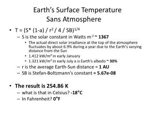
Chapter 3. IPCC report Observations: Surface and Atmosphere Climate Change. 1. Changes in Surface Climate: Temperature (T ) 2. Changes in Surface Climate: Precipitation (P), Drought and Surface Hydrology. Land-Surface Air Temperature.

E N D
Chapter 3. IPCC report Observations: Surface and Atmosphere Climate Change
1. Changes in Surface Climate:Temperature (T) 2. Changes in Surface Climate: Precipitation (P), Drought and Surface Hydrology
Land-Surface Air Temperature Figure 3.1. Annual anomalies of global land-surface air temperature (°C), 1850 to 2005, relative to the 1961 to 1990 mean for CRUTEM3 updated from Brohan et al. (2006). The smooth curves show decadal variations (see Appendix 3.A). The black curve from CRUTEM3 is compared with those from NCDC (Smith and Reynolds, 2005; blue), GISS (Hansen et al., 2001; red) and Lugina et al. (2005; green).
Max, Min T & Diurnal Temperature Range(DTR) Figure 3.2. Annual anomalies of maximum and minimum temperatures and DTR(°C) relative to the 1961 to 1990 mean, averaged for the 71% of global land areas where data are available for 1950 to 2004. The smooth curves show decadal variations (see Appendix 3.A). Adapted from Vose et al. (2005a).
Urban Heat Island (UHI) & Land Use Effects • UHI and changes in land use can be important for DTR at the regional scale • The global land warming trend is unlikely to be influenced significantly by increasing urbanization. Figure 3.3. Anomaly (°C) time series relative to the 1961 to 1990 mean of the full US Historical Climatology Network (USHCN) data (red), the USHCN data without the 16% of the stations with populations of over 30,000 within 6 km in the year 2000 (blue), and the 16% of the stations with populations over 30,000 (green). The full USHCN set minus the set without the urban stations is shown in magenta. Both the full data set and the data set without the high-population stations had stations in all of the 2.5° latitude by 3.5° longitude grid boxes during the entire period plotted, but the subset of high-population stations only had data in 56% of these grid boxes. Adapted from Peterson and Owen (2005).
SST and Marine Air Temperature Figure 3.4. (a) Annual anomalies of global SST (HadSST2; red bars and blue solid curve), 1850 to 2005, and global NMAT (HadMAT, green curve), 1856 to 2005, relative to the 1961 to 1990 mean (°C) from the UK Meteorological Office. The smooth curves show decadal variations . The dashed black curve shows equivalent smoothed SST anomalies from the TAR. (b) Smoothed annual global SST anomalies, relative to 1961 to 1990 (°C), from HadSST2 (blue line, as in (a)), from NCDC (Smith et al., 2005; red line) and from COBE-SST (Ishii et al., 2005; green line). The latter two series begin later in the 19th century than HadSST2. (c,d) As in (a) butfor the NH and SH showing only the UKMO series. It is likely to have arisen partly from closely spaced multiple El Niño events and also due to the warm phase of the Atlantic Multi-decadal Oscillation (AMO).
Land and Sea Combined T Figure 3.6. Global and hemispheric annual combined land- surface air temperature and SST anomalies (°C) (red) for 1850 to 2006 relative to the 1961 to 1990 mean,along with 5 to 95% error bar ranges, from HadCRUT3 .The smooth blue curves show decadal variations Figure 3.7. Annual temperature anomalies (°C) up to 2005, relative to the 1961 to 1990 mean (red) with 5 to 95% error bars. The tropical series (middle) is combined land-surface air temperature and SST from HADCRUT3 The polar series (top and bottom) are land-only from CRUTEM3, because SST data are sparse and unreliable in sea ice zones. The smooth blue curves showdecadal variations
Global Mean T is Increasing Annual global mean observed temperatures1 (black dots) along with simple fi ts to the data. The left hand axis shows anomalies relative to the 1961 to 1990 average and the right hand axis shows the estimated actual temperature (°C). Linear trend fi ts to the last 25 (yellow), 50 (orange), 100 (purple) and 150 years (red) are shown, and correspond to 1981 to 2005, 1956 to 2005, 1906 to 2005, and 1856 to 2005, respectively.
Spatial Trend Patterns of T(Annual) • In Asia, NW of North America, SH mid-latitude oceans and Brazil, T has a strong increasing trend Figure 3.9. Linear trend of annual temperatures for 1901 to 2005 (left; °C per century) and 1979 to 2005 (right; °C per decade). Areas in grey have insuffi cient data to produce reliable trends. Trends signifi cant at the 5% level are indicated by white + marks.
Spatial Trend Patterns of T(Seasonal) Figure 3.10. Linear trend of seasonal MAM, JJA, SON and DJF temperature for 1979 to 2005 (°C per decade). The dataset used was produced by NCDC from Smith and Reynolds (2005). Trends signifi cant at the 5% level are indicated by white + marks.
Spatial Trend Patterns of T(Surface vs Troposphere) Patterns of linear global temperature trends from 1979 to 2005 estimated at the surface (left), and for the troposphere (right) from the surface to about 10 km altitude,from satellite records. Grey areas indicate incomplete data. • Spatially uniform warming in troposphere • Surface T changes more clearly between land and ocean.
Changes in Surface Climate: Precipitation (P), Drought and Surface Hydrology
Global Annual Land P Anomalies • Increased till the 1950s • Decreased 1950s-1990s • Recovered in recent years Figure 3.12. Time series for 1900 to 2005 of annual global land precipitation anomalies (mm) from GHCN with respect to the 1981 to 2000 base period. The smooth curves show decadal variations (see Appendix 3.A) for the GHCN (Peterson and Vose, 1997), PREC/L (Chen et al., 2002), GPCP (Adler et al., 2003), GPCC (Rudolfet al., 1994) and CRU (Mitchell and Jones, 2005) data sets.
Spatial Patterns of P trends 1901-2005 • Sahel • South America • NE of northAmerica 1979-2005 Figure 3.13. Trend of annual land precipitation amounts for 1901 to 2005 (top, % per century) and 1979 to 2005 (bottom, % per decade), using the GHCN precipitation data set from NCDC. The percentage is based on the means for the 1961 to 1990 period. Areas in grey have insuffi cient data to produce reliable trends. Trends signifi cant at the 5% level are indicated by black + marks.
How does snow and heavy Precipitation events change? Under the global warming circumstances: • More P now falls as rain rather than snow in northern regions, which corresponding to the longer liquid P season. • Widespread increases in heavy precipitation events (Due to the increased water-holding capacity of the air)
Precipitation in Urban Areas • Urban effects can lead to increased precipitation during the summer months within and 50 to 75 km downwind of the city • Suggested mechanisms for urban-induced rainfall include: (1) Enhanced convergence due to increased surface roughness (2) Destabilisation due to UHI thermal perturbation of the boundary layer and resulting downstream translation of the UHI circulation or UHI-generated convective clouds (3) Enhanced aerosols for cloud condensation nuclei sources (4) Bifurcating or diverting of precipitating systems by the urban canopy or related processes
Drought • Palmer Drought Severity Index (PDSI) • Index of drought and measures the cumulative deficit in surface land moisture • Less than -0.5 means drought
PDSI pattern and time series • Eastern North& South America, northern Eurasia are getting wetter • Africa is getting dryer, especially in Sahel • Very dry areas have more than doubled since the 1970s. The spatial pattern (top) of the monthly (PDSI for 1900 to 2002. The The lower panel shows how the sign and strength of this pattern has changed since 1900. Red and orange areas are drier (wetter) than average and blue and green areas are wetter (drier) than average when the values shown in the lower plot are positive (negative).The smooth black curve shows decadal variations. The time series approximately corresponds to a trend, and this pattern and its variations account for 67% of the lineartrend of PDSI from 1900 to 2002 over the global land area.
Consistency and Relationship between T&P • In the warm season over land, higher T accompanies lower P and vice versa. • At latitudes polarward of in winter, P and T are positive correlated. • In regions , where the ocean conditions drive the air, P and T have a positive correlation
Observations in Free Atmosphere 1940 - 1958 : Radiosonde 1978 : Microwave Satellite Unit (MSU) Mid 1998 - Advanced MSU ( 20 Channels compared to 4 of MSU) Troposphere and stratosphere temperatures Clouds Water vapor Atmospheric general circulation Teleconnection patterns
Satellite observations revolutionize our understanding Figure 3.16. Vertical weighting functions (grey) depicting the layers sampled by satellite MSU measurements and their derivatives, and used also for radiosonde and reanalysis records. The right panel schematically depicts the variation in the tropopause (that separates the stratosphere and troposphere) from the tropics (left) to the high latitudes (right). The fourth panel depicts T4 in the lower stratosphere, the third panel shows T2, the second panel shows the troposphere as a combination of T2 and T4 (Fu et al., 2004a) and the first panel shows T2LT from the UAH for the low troposphere. Adapted from Karl et al. (2006).
Observations show stratosphere cooling and warming of troposphere • Radiosonde observations have some very strong limitations and not so dense network of data, while satellites have some time sampling and calibration errors • All the modes of data show stratospheric cooling and tropospheric warming Figure 3.17. Observed surface and upper-air temperature anomalies (°C). (A) Lower stratospheric T4, (B) Tropospheric T2, (C) Lower tropospheric T2LT, from UAH, RSS and VG2 MSU satellite analyses and UKMO HadAT2 and NOAA RATPAC radiosonde observations; and (D) Surface records from NOAA, NASA/GISS and UKMO/CRU (HadCRUT2v). All time series are monthly mean anomalies relative to the period 1979 to 1997 smoothed with a seven-month running mean filter. Major volcanic eruptions are indicated by vertical blue dashed lines. Adapted from Karl et al. (2006).
Extratopical troposphere warming is unprecedented Figure 3.18. Linear temperature trends (°C per decade) for 1979 to 2004 for the globe (left) and tropics (20°N to 20°S; right) for the MSU channels T4 (top panel) and T2 (second panel) or equivalent for radiosondes and reanalyses; for the troposphere (third panel) based on T2 with T4 used to statistically remove stratospheric influences (Fu et al., 2004a); for the lower troposphere (fourth panel) based on the UAH retrieval profile; and for the surface (bottom panel). Surface records are from NOAA/NCDC (green), NASA/GISS (blue) and HadCRUT2v (light blue). Satellite records are from UAH (orange), RSS (dark red) and VG2 (magenta); radiosonde-based records are from NOAA RATPAC (brown) and HadAT2 (light green); and atmospheric reanalyses are from NRA (red) and ERA-40 (cyan). The error bars are 5 to 95% confidence limits associated with sampling a finite record with an allowance for autocorrelation. Where the confidence limits exceed –1, the values are truncated. ERA-40 trends are only for 1979 to August 2002.Data from Karl et al. (2006; D. Seidel courtesy of J. Lanzante; and Christy).
Tropics show low linear trends and while NH extratropics exhibit highest Figure 3.19. Linear tropospheric temperature trends (°C per decade) for 1979 to 2005 from RSS (based on T2 and T4 adjusted as in Fu et al., 2004a). Courtesy Q. Fu.
Multi-decadal water vapor analyses show trends Figure 3.21. The radiative signature of upper-tropospheric moistening is given by upward linear trends in T2−T12 for 1982 to 2004 (0.1 ºC per decade; top) and monthly time series of the global-mean (80°N to 80°S) anomalies relative to 1982 to 2004 (ºC) and linear trend (dashed; bottom). Data are from the RSS T2 and HIRS T12 (Soden et al., 2005). The map is smoothed to spectral truncation T31 resolution. Figure 3.20. Linear trends in precipitable water (total column water vapour) in % per decade (top) and monthly time series of anomalies relative to the 1988 to 2004 period in % over the global ocean plus linear trend (bottom), from RSS SSM/I (updated from Trenberth et al., 2005a). • However we do not posses reliable records of long-term water vapor trends throughout the planet for all the layers
No detectable multi-decadal cloud trends on land globally • Largest uncertainty is realizations of cloud cover in association with Greenhouse gas warming • Different peer-reviewed studies contradict each other about change of low-level content, while agree decline of high clouds qualitatively Figure 3.22. Annual total land (excluding the USA and Canada) cloud cover (black) and precipitation (red) anomalies from 1976 to 2003 over global (60°S–75°N), NH and SH regions, with the correlation coefficient (r) shown at the top. The cloud cover is derived by gridding and area-averaging synoptic observations and the precipitation is updated from Chen et al. (2002). Typical 5 to 95% error bars for each decade are estimates using inter-grid-box variations (from Dai et al., 2006). • Local cloud trends vary widely over different parts on land • High clouds decline globally in 1990s compared to 1980s (ISCCP)
Net tropical radiative forcing show increased atmospheric warming Figure 3.23. Tropical mean (20°S to 20°N) TOA flux anomalies from 1985 to 1999 (W m–2) for LW, SW, and NET radiative fluxes [NET = −(LW + SW)]. Coloured lines are observations from ERBS Edition 3_Rev1 data from Wong et al. (2006) updated from Wielicki et al. (2002a), including spacecraft altitude and SW dome transmission corrections. • This means that feedback of clouds at the top of the atmosphere is warming (ERBS and ISCCP) • However our understanding of low-clouds could change the TOA net in the table above
So far we observed that Surface temperature show increasing trends Total column water vapor show increasing trends Cloud cover changes An obvious question can arise about what happens to the atmospheric boundary layer?
ERA-40 planetary boundary layer (PBL) heights show sensitivity to large-scale circulation in Dec-Jan-Feb • Data considered: 1959-2002 Dec-Jan-Feb average PBL heights • T0 = mean PBL height between 1981-2002 does not statistically differ from 1959-1980 Note: Only 5% significant levels shown for t-test
PBL heights show significant changes possibly to local hydrometeorological quantities in Jun-Jul-Aug • Most parts of north America and some parts in Eurasia show significant PBL height changes Note: Only 5% significant levels shown for t-test
Geopotential height (GPH) trends show increased baroclinic activity more storminess Figure 3.24. Linear trends in ERA-40 700 hPa geopotential height from 1979 to 2001 for DJF (top left and bottom right) and JJA (bottom left and top right), for the NH (left) and SH (right). Trends are contoured in 5 gpm per decade and are calculated from seasonal means of daily 1200 UTC fields. Red contours are positive, blue negative and black zero; the grey background indicates 1% statistical significance using a standard least squares F-test and assuming independence between years. • Strong contrasts between mid and high latitudinal geopotential heights in each winter hemisphere is depicted
Decreasing trend in persistent blocking in north Atlantic and no trend in short lived blocking Technical detail: The above picture shows a random blocking event in northern Atlantic. Such high pressure blockings are commonly known to exist in northern Pacific too. • Negative NAO is correlated with increased blocking events in north Atlantic • In north Pacific region during El Nino years, the blocking is significantly weaker • Much harder to define any trend in Sourthern hemisphere
Interannual GPH standard deviation shows significant changes with respect to 1976/77 climate shift 5% significance regions are shaded Technical details: ERA40 700 hpa data is used for the analysis. All DJF values are averaged to 1 value at each grid point. Therefore each grid point has 24 values for 1977-01 and 19 for 1958-76.
Intraseasonal GPH standard deviation shows Post 1976 climate has more variability
Wave number-frequency domain for different climate regimes show distinguished persistent wave density at transient planetary wave scale • 1958-76 GPH show spectral density spread quasi-evenly from wave numbers 3-5, while 1977-01 climate show concentrated at wave number four Technical details:700 hpa GPH data from ERA40 is considered for this analysis. Space-time structure of the variable is transformed to wave number-frequency. The color bar shows in units of 103 m2 day-1. Please see Straus and Shulka (1981): Space-time spectral structure of a GLAS general circulation model and a comparison with observations.
Net propagation tendency (NPT) calculations show strong relative eastward propagation in 1977-01 regime Could be attributed to decrease in long- term persisting blocking events Technical details: NPT (= (Eastward density-Westward density)/(Eastward density+Westward density)) calculated for both pre and post 1976 regimes. NPT value of 1.0 meanss pure east ward propagation. The above figure shows the difference between post and pre 1976 values, that is relative eastward propagation tendency.
Atypical sudden stratospheric warming is detected in recent years • Starting from late 1990s more neutral states of NAM is observed • In southern hemisphere only one such sudden warming is observed in 2002
Significant wave heights support increased storminess in NH extratrpoics Figure 3.25. Estimates of linear trends in significant wave height (cm per decade) for regions along the major ship routes of the global ocean for 1950 to 2002. Trends are shown only for locations where they are significant at the 5% level. Adapted from Gulev and Grigorieva (2004). Technical detail: Significant wave height can be approximated as average of top one third of waves. For a comprehensive discussion see: http://www.ndbc.noaa.gov/wavecalc.shtml
What are preferred climate patterns of planet earth? Teleconnection patterns - PNA and NAO Figure 3.26. The PNA (left) and NAO (right) teleconnection patterns, shown as one-point correlation maps of 500 hPa geopotential heights for boreal winter (DJF) over 1958 to 2005. In the left panel, the reference point is 45°N, 165°W, corresponding to the primary centre of action of the PNA pattern, given by the + sign. In the right panel, the NAO pattern is illustrated based on a reference point of 65°N, 30°W. Negative correlation coefficients are dashed, and the contour increment is 0.2. Adapted from Hurrell et al. (2003).
SOI index shows significant ENSO changes since 1976/77 climate shift Figure 3.27. Correlations with the SOI, based on normalised Tahiti (149.6°W, 17.5°S) minus Darwin (130.9°E, 12.4°S) sea level pressures, for annual (May to April) means for sea level pressure (top left) and surface temperature (top right) for 1958 to 2004, and GPCP precipitation for 1979 to 2003 (bottom left), updated from Trenberth and Caron (2000). The Darwin-based SOI, in normalized units of standard deviation, from 1866 to 2005 (Können et al., 1998; lower right) features monthly values with an 11-point low-pass filter, which effectively removes fluctuations with periods of less than eight months (Trenberth, 1984).The smooth black curve shows decadal variations (see Appendix 3.A). Red values indicate positive sea level pressure anomalies at Darwin and thus El Niño conditions.
No discernible multi-decadal trend in Pacific Decadal Oscillation (PDO) index with respect to 1976/77 climate shift Figure 3.28. Pacific Decadal Oscillation: (top) SST based on the leading EOF SST pattern for the Pacific basin north of 20°N for 1901 to 2004 (updated; see Mantua et al., 1997; Power et al., 1999b) and projected for the global ocean (units are nondimensional); and (bottom) annual time series (updated from Mantua et al., 1997). The smooth black curve shows decadal variations • Prediction of future trends in PDO enhances our understanding of high-latitude continental temperatures
PDO may not be an independent phenomenon by itself Continental Alaska temperatures are highly correlated with PDO changes Source: Hartmann and Wendler, 2005: The significance of the 1976 climate shift in the climatology of Alaska, J. Clim. 18:4824-2005
A brief introduction on NAO • Generally taken as SLP difference between Reykjavik (most northern capital of a nation) and Ponta Delgada (belongs to Portugal)) • NAO has huge impact on the day-to-day as well as intraseasonal variability over north Atlantic region (much of north America, Europe north Asia) Positive phase Negative phase Source: http://www.ldeo.columbia.edu/res/pi/NAO/
NAO significantly influences westerlies and NH precipitation Figure 3.30. Changes in winter (December–March) surface pressure, temperature, and precipitation corresponding to a unit deviation of the NAO index over 1900 to 2005. (Top left) Mean sea level pressure (0.1 hPa). Values greater than 0.5 hPa are stippled and values less than −0.5 hPa are hatched. (Top right) Land-surface air and sea surface temperatures (0.1°C; contour increment 0.2°C). Temperature changes greater than 0.1°C are indicated by stippling, those less than –0.1°C are indicated by hatching, and regions of insufficient data (e.g., over much of the Arctic) are not contoured. (Bottom left) Precipitation for 1979 to 2003 based on GPCP (0.1 mm per day; contour interval 0.6 mm per day). Stippling indicates values greater than 0.3 mm per day and hatching values less than –0.3 mm per day. Adapted and updated from Hurrell et al. (2003).
A long time-series of NAO and NAM trends show significant changes Figure 3.31. Normalised indices (units of standard deviation) of the mean winter (December–March) NAO developed from sea level pressure data. In the top panel, the index is based on the difference of normalised sea level pressure between Lisbon, Portugal and Stykkisholmur/Reykjavik, Iceland from 1864 to 2005. The average winter sea level pressure data at each station were normalised by dividing each seasonal pressure anomaly by the long-term (1864 to 1983) standard deviation. In the middle panel, the index is the principal component time series of the leading EOF of Atlantic-sector sea level pressure. In the lower panel, the index is the principal component time series of the leading EOF of NH sea level pressure. The smooth black curves show decadal variations (see Appendix 3.A). The individual bar corresponds to the January of the winter season (e.g.,1990 is the winter of 1989/1990). Updated from Hurrell et al. (2003); see http://www.cgd.ucar.edu/cas/jhurrell/indices.html for updated time series.
Current NAO and NAM indices show persistent positive trend Source: http://www.cgd.ucar.edu/cas/jhurrell/indices.info.html#naostatseas
Both tropical and extratropical Atlantic show significant multidecadal trends Figure 3.33. Atlantic Multi-decadal Oscillation index from 1850 to 2005 represented by annual anomalies of SST in the extratropical North Atlantic (30–65°N; top), and in a more muted fashion in the tropical Atlantic (10°N –20°N) SST anomalies (bottom). Both series come from HadSST2 (Rayner et al., 2006) and are relative to the 1961 to 1990 mean (°C). The smooth blue curves show decadal variations). • Thermohaline circulation might be reason for Atlantic multi decadal trend • Effects include hurricane activity, Sahel droughts, precipitation anomalies over Caribbean, north America and Europe
Aleutian low is strengthened, while Indian ocean SSTs show significant multidecadal trend Figure 3.29. (Left) Time series of the NPI (sea level pressure during December through March averaged over the North Pacific, 30°N to 65°N, 160°E to 140°W) from 1900 to 2005 expressed as normalised departures from the long-term mean (each tick mark on the ordinate represents two standard deviations, or 5.5 hPa). This record reflects the strength of the winter Aleutian Low pressure system, with positive (negative) values indicative of a weak (strong) Aleutian Low. The bars give the winter series and the smooth black curves show decadal variations (see Appendix 3.A). Values were updated and extended to earlier decades from Trenberth and Hurrell (1994). (Right) As above but for SSTs averaged over the tropical Indian Ocean (10°S–20°N, 50°E –125°E; each tick mark represents two standard deviations, or 0.36°C). This record has been inverted to facilitate comparison with the top panel. The dashed vertical lines mark years of transition in the Aleutian Low record (1925, 1947, 1977). Updated from Deser et al. (2004). • There is a strong correlation between Aleutian low and Indian Ocean SST
SAM index shows increased cyclonic activity and a slight warming around Peninsula region Figure 3.32. (Bottom) Seasonal values of the SAM index calculated from station data (updated from Marshall, 2003). The smooth black curve shows decadal variations. (Top) The SAM geopotential height pattern as a regression based on the SAM time series for seasonal anomalies at 850 hPa (see also Thompson and Wallace, 2000). (Middle) The regression of changes in surface temperature (°C) over the 23-year period (1982 to 2004) corresponding a unit change in the SAM index, plotted south of 60°S. Values exceeding about 0.4°C in magnitude are significant at the 1% significance level (adapted from Kwok and Comiso, 2002b).