Quantitative Decision Techniques: An Overview of Operations Research
This text provides a detailed insight into Operations Research (OR) and its application of scientific methods to solve complex managerial decision problems. It covers mathematical modeling, mathematical programming, optimization models, decision models, quantitative analysis, and a seven-step model building process in management science.

Quantitative Decision Techniques: An Overview of Operations Research
E N D
Presentation Transcript
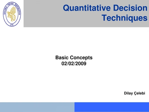
Quantitative Decision Techniques Basic Concepts 02/02/2009 Dilay Çelebi
OPERATIONS RESEARCH 1. MS/OR is the application of scientific methods, techniques and tools to problems involving the operations of systems so as to provide those in control of the operations with optimum solutions to the problems. 2. MS/OR is the application of the scientific method to the study of the operations of large, complex organizations or activities. 3. MS/OR is the application of the scientific method to the analysis and solution of managerial decision problems. OR deals with making decisions based onmodeling. Its origins date back to the second world war!
MATHEMATICAL MODELING A model is a selective abstraction of reality* A model is a representation of a situation** A mathematical model is an abstract mathematical representation of a problem situation. Mathematical Programming(Modeling), MP, is the use of mathematical models, particularly optimizing models, to assist in taking decisions *Introductory Management Science, F.J. Gould, G.D. Eppen, C.P. Schmidt, 1993. **Quantitative Analysis for Management, 9th Edition, Barry Render, Ralph M. Stair, M. Hanna, 2006.
120 km City B City A V=30 km/hour Quantitative Models Incorporate enough detail into your model so that • The result meets your needs • You can solve it in the time you have to devote to the process • QM uses mathematics to represent the relationship between data of interest. • Data should be quantifiable! How long does it take to get to city B from city A? A model usually simplifies reality Introductory Management Science, F.J. Gould, G.D. Eppen, C.P. Schmidt, 1993.
120 km City B City A V=? Stop at Restaurant? Decision Models Decision Models • Selectively describe the environment • Designate decision variables • Designate objectives • Defined by constraints Decision Variables Speed, stop points, road • Objectives • Minimize total travel time • Be in City B around 9 • Constraints • Max speed of car • Number of hours in therest. Introductory Management Science, F.J. Gould, G.D. Eppen, C.P. Schmidt, 1993.
OptimizationModels The goal of an optimization model is to make some function of the decision variables as large or as small as possible.* Optimization means "the action of finding the best solution". Optimization modeling, is a branch of mathematical modeling which is concerned with finding the best solution to a problem EXAMPLES Profit maximization Cost minimization Minimization of waiting times Maximum use of capacity Minimum working hours *Introductory Management Science, F.J. Gould, G.D. Eppen, C.P. Schmidt, 1993.
QUANTITATIVE ANALYSIS Quantitative Analysis Decision Making Process Conflicting Viewpoints Problem Definition Problem Definition Assumptions and Boundaries Search for Alternatives Observations Decision Variables Mathematical Relationships Constraints Model Construction Developing a Solution Testing the Solution Evaluation Selection of Best Alternative Presentation Implementation Choice Analyzing the Results Introductory Management Science, F.J. Gould, G.D. Eppen, C.P. Schmidt, 1993. Fundamentals of Management Science, Efraim Turban, Jack R. Meredith, 1981
THE SEVEN - STEP MODEL BUILDING PROCESS When quantitative approach is used to solve a problem of an organization, the following seven step model building procedure should be followed. Step 1. Formulate the Problem First define the organization's problem! Defining the problem includes specifying the organization's objectives and the parts of the organization (or system) that must be studied before the problem can be solved. Step 2. Observe the System Collect data to estimate the value of parameters that affect the organization's problem. These estimates are used to develop (in Step 3) and evaluate (in Step 4) a mathematical model of the organization's problem. Introduction to Management Science, 9th Edition, Taylor B.W., 2007.
THE SEVEN - STEP MODEL BUILDING PROCESS Step 3. Formulate a Mathematical Model of the Problem Develop a mathematical model (in other words an idealized representation) of the problem. Step 4. Verify the Model and Use the Model for Prediction Try to determine if the mathematical model developed in Step 3 is an accurate representation of reality. Even if a model is valid for the current situation, we must be aware of blindly applying it. Step 5. Select a Suitable Alternative Given a model and a set of alternatives, choose the alternative that best meets the organization's objectives. There may be more than one! Introduction to Management Science, 9th Edition, Taylor B.W., 2007.
THE SEVEN - STEP MODEL BUILDING PROCESS Step 6. Present the Results and Conclusions of the Study to the Organization Present the model and the recommendations from Step 5 to the decision making individual or group. After presenting the results, you may find that the organization does not approve of the recommendations. This may result from incorrect definition of the organization’s problem or from failure to involve decision maker from the start of the project. In this case, you should return to Step 1, 2, or 3. Step 7. Implement and Evaluate Recommendation Implement the study. The system must be constantly monitored (and updated dynamically as the environment changes) to ensure that the recommendations enable the organization to meet its objectives. Introduction to Management Science, 9th Edition, Taylor B.W., 2007.
MANAGEMENT SCIENCE TECHNIQUES Deterministic models are models which donot contain the element of probability.These are primarily optimization models. • Linear Programming • linear objective function – min/max • linear constraints • Integer LP, Binary LP, Mixed Integer LP • Nonlinear Programming • nonlinear objective function and/or • nonlinear constraints
MANAGEMENT SCIENCE TECHNIQUES • Distribution Models • special type of LP problems (special structure of model) • transportation problem • assignment problem • Multicriteria Decision Making • multiple criteria • compromise • limited/unlimited number of alternatives • goal programming
MANAGEMENT SCIENCE TECHNIQUES Stochastic models are models whichcontain the element of probability. • Inventory Models • when to order? • how much to order? • Waiting Line Models (Queuing Models) • servers, customers • goal – optimal number of server • Computer Simulation • computer experiments with models • complex systems
Model Reality MATHEMATICAL MODELS Finding a proper balance between the level of simplification of the model and the good representation of reality. ___________________________________________________________________________ Operations Research Jan Fábry
LINEAR PROGRAMMING The word linear comes from the Latin word linearis, which means created by lines LINEAR FUNCTION: Each term is either a constant or the product of a constant times the first power of a variable. These are NOT linear functions: These are linear functions:
LINEAR PROGRAMMING A linear programming problem (LP) is an optimization problem for which we do the following: • We attempt to maximize (or minimize) a linear function of the decision variables. The function that is to be maximized or minimized is called the objective function. A function f (x1, x2, …….xn) of x1, x2,…….xn is a linear function if and only if for some set of constants c1, c2, …..cn , f (x1, x2,…..xn) = c1x1 + c2x2 + c3x3+……..cnxn. For example, f (x1, x2)= 2x1 + x2 is a linear function of x1, x2, but f (x1, x2)= 2x1x2 is not a linear function of x1, x2.
LINEAR PROGRAMMING 2. The values of decision variables must satisfy a set of constraints. Each constraint must be a linear equation or a linear inequality. For any linear function f (x1, x2, …….xn) and any number b, the inequalities f (x1, x2, …….xn) b and f (x1, x2, …….xn) ) b are linear inequalities. For example, 2x1 + x2 = 100 is a linear equation, 2x1 + x2 ≤ 20 or x1 + 5x2 ≥40 are linear inequalities, but x1x2 ≥ 40 or x12x2 ≤ 20 are not linear inequalities.
LINEAR PROGRAMMING 3. A sign restriction is associated with each variable. For any variable xi , the sign restriction specifies either that xi must be nonnegative (xi ≥ 0) or that xi may be unrestricted in sign (urs). (An LP with unrestricted-in-sign variables is transformed into an LP in which all variables are required to be nonnegative because nonnegativity restrictions are essential for the development of the solution algorithm of the LP).
LINEAR PROGRAMMING • The steps in formulating a linear program follow*: • Completely understand the managerial problem being faced • Identify the objective and the constraints • Define the decision variables • Use the decision the variables to write mathematical expressions for the objective function and the constraints. Render et al., pp. 236
ELEMENTS OF LINEAR PROGRAMMING • Decision Variables: In any linear programming model the decision variables should completely describe the decisions to be made (xi) . • Objective Function:In any linear programming problem, the decision maker wants to maximize (usually revenue or profit) or minimize (usually costs) some function of the decision variables. The function to be maximized or minimized is called the objective function (Zmin or Zmax). • The coefficient of a variable in the objective function is called the objective function coefficientof the variable (cj). The coefficients represent the contribution of one unit of variable to the company’s goal.
Decision Variables Objective Function Complete mathematical statement of the LP problem Zmax = 3 x1+ 2x2 Subject to (s.t.) 2x1 + x2 ≤ 100 x1 + x2 ≤ 80 x1 ≥40 x1 ≥ 0 x2 ≥ 0
ELEMENTS OF LINEAR PROGRAMMING • Constraints • Restrictions on the values of decision variables • Right hand side of a constraints (bi) represent the quantity of a resource that is available. For a constraint to be reasonable, all term in the constraint must have the same units. Otherwise, the constraint will not have any meaning. • The coefficients of the decision variables in the constraints are called technological coefficients (aij). Technological coefficients often reflect the technology used to produce different product.
Complete mathematical statement of the LP problem Decision Variables Zmax = 3 x1+ 2x2 Subject to (s.t.) 2x1 + x2 ≤ 100 x1 + x2 ≤ 80 x1 ≥40 x1 ≥ 0 x2 ≥ 0 Objective Function Constraints
Decision Variables General Form of LP Problems Objective Function Constraints
Formulating Linear Programs • Choose the variables for the LP by considering the fundamental processes that the modeler can control. • Determine the objective function by • Finding how much each variable contributes to the objective per unit of that variable used • Adding the contributions of each of the variables to obtain the (linear) objective. • Determining whether the objective is to be maximized or minimized.
Formulating Linear Programs • Determine the constraints of the problem, by formalizing the restrictions on the variables imposed by the modeler. Again, for each constraint: • determine the demand of each variable for the resource associated with that constraint • add the demands of each of the variables to obtain the total demand for that resource • determine whether that resource constitutes an upper bound on the total demand (≤constraint) a lower bound on the total demand (≥constraint) or an exact requirement on the total demand (= constraint). • Be sure to include the nonnegativity constraints if the variables require this.
PRODUCTION MIX PROBLEM A clothier makes coats and slacks. The two resources requiredare wool cloth and labor. The clothier has 150 square yards of wooland 200 hours of labor available. Each coat requires 3 square yardsof wool and 10 hours of labor, whereas each pair of slacks requires5 square yards of wool and 4 hours of labor. The profit for a coatis $50, and the profit for slacks is $40. The clothier wants todetermine the number of coats and pairs of slacks to make so thatprofit will be maximized.
PRODUCTION MIX PROBLEM A jewelry store makes necklaces and bracelets from gold and platinum. The store has 18 ounces of gold and 20 ounces of platinum. Each necklace requires 3 ounces of gold and 2 ounces of platinum, whereas each bracelet requires 2 ounces of gold and 4 ounces of platinum. The demand for bracelet is no more than four. A necklace earns $300 in profit and a bracelet, $400. The store wants to determine the number of necklaces and bracelets to make in order to maximize profit.
Assumptions of LP Proportionality and Additivity Assumptions of Linear Programming The fact that the objective function for an LP must be a linear function of the decision variables has two implications. 1. The contribution of the objective function from each decision variable is proportional to the value of the decision variable. For example, the contribution of the objective function from making four soldiers (4 * 3 = $12) is exactly four times the contribution to the objective function from making one soldier ($3). 2. The contribution to the objective function for any variable is independent of the values of the other decision variables. For example, no matter what the value of the X2, the manufacture of X1 soldierswill always contribute 3X1 to the objective function.
Analogously, the fact that each LP constraint must be a linear inequality or alinear equation has two implications. 1. The contribution of each variable to the left-hand side of each constraint is proportional to the value of the variable. For example, it takes exactly three times as many finishing hours (2 * 3 = 6 finishing hours) to manufacture three soldiers as it takes to manufacture one soldier (2 finishing hours). 2. The contribution of a variable to the left-hand side of each constraint is independent of the values of the variable. For example, no matter what the value of X1, the manufacture of X2 trains uses 1X2 finishing hours and 1X2 carpentry hours.
The first implication given in each list is called the Proportionality Assumption of Linear Programming. Implication 2 of the first list implies that the value of the objective function is the sum of the contribution of from individual variables, and implication 2 of the second list implies that the left-hand side of each constraint is the sum of the contributions from each variable. For this reason, the second implication in each list is called the Additivity Assumption of Linear Programming.
The Divisibility Assumption The Divisibility Assumption requires that each decision variable be allowed to assume fractional values. For example, in the Giapetto’s Problem, The Divisibility Assumption implies that it is acceptable to produce 1.5 soldiers or 1.63 trains. Since Giapetto cannot actually produce a fractional number of trains or soldiers, the Divisibility Assumption is not satisfied in the Giapetto Problem. A linear programming problem in which some or all of the variables must be nonnegative integers is called an integer programming problem.
The Certainty Assumption The Certainty Assumption is that each parameter (objective function coefficient, right-hand side, and technological coefficient) is known with certainty. If we were unsure of the exact amount of carpentry and finishing hours required to build a train, the Certainty Assumption would be violated.
OTHER PROBLEMS • Blending Problem - The Holiday Meal Turkey Ranch • Media Selecting Problem - Dorian Auto
REFERENCES • Introduction to Management Science, 9th Edition, Taylor B.W., Prentice Hall, New Jersey, 2007. ISBN: 0-13-1966133-0, ITU Library Number: T56.T39.1990/T56.T39 1986. • Quantitative Analysis for Management, 9th Edition, Barry Render, Ralph M. Stair, M. Hanna, Prentice Hall, New Jersey, 2006. ISBN: 0-13-153688-5, ITU Library Number: T56.R46 2006. • Fundamentals of Management Science, Efraim Turban, Jack R. Meredith, Plano, Tex. : Business Publications, 1981. ISBN: 025602393X, ITU Library Number: HD30.23.T87 1981 • Introductory Management Science, F.J. Gould, G.D. Eppen, C.P. Schmidt, Englewood Cliffs, N.J. : Prentice Hall, c1993. ISBN:0134864409, ITU Library Number: HD30.25.G68 1993.