Download
1 / 37
370 likes | 453 Vues
This survey explores recent German research on sprat, focusing on stock reproductive potential, early life stages, feeding, IBM modeling, and more. Projects such as Baltic CORE and STORE delve into stock size, recruitment, and adult reproduction biology of Baltic sprat. Discover the findings related to larval abundance, adult reproduction, and vertical distribution of sprat in the Baltic and North Sea. Uncover the significant factors influencing sprat fecundity, adult reproduction, and stock recruitment. This comprehensive overview sheds light on the complexities of sprat ecology and management.

E N D
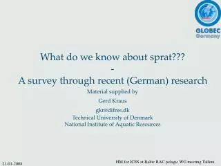
What do we know about sprat??? - A survey through recent (German) research Material supplied by Gerd Kraus gkr@difres.dk Technical University of Denmark National Institute of Aquatic Resources HM for ICES at Baltic RAC pelagic WG meeting Tallinn
EU-funded Baltic CORE (Cod recruitment in the Baltic) and STORE (Environmental and fisheries influences on fish stock recruitment in the Baltic Sea) projects: -stock reproductive potential (viable EP) -Early life stages & Hydrography -Feeding, growth, survival -IBM modeling -Preator-prey interactions -Recruitment modelling & management aspects The German Globec Project (Trophic Interactions between Zooplankton and Fish under the Influence of Physical Processes) focussed on: -sprat & (herring) -copepods as key prey species -experiments, process studies, field sampling, process- to 3-D ecosystem modeling -Analyses restricted to Globec years (2002-2005) German Science Foundation funded project “Resolving Trophodynamic Consequences of Climate Change”targets sprat in the Baltic and North Sea: -time series analyses -Experiments; Process models -Coupled Tropho-Hydrodynamic modeling HM for ICES at Baltic RAC pelagic WG meeting Tallinn
German Bight Bornholm Basin German Globec • • Funded for 6 years (2002 – 2007) • 8 Institutions (incl. Difres) • • 11 sub-projects • • 80 scientists and technicians • • 12 PhD students • • 13 student projects (diploma) • 48 cruises in Baltic and North Sea • 736 days at Sea HM for ICES at Baltic RAC pelagic WG meeting Tallinn
Background / Hypotheses • Adult reproduction biology and distribution • Early life stage biology and relevance of early life processes for recruitment • Modeling approches -Hydrodynamic -Ecosystem -IBM -Coupling HM for ICES at Baltic RAC pelagic WG meeting Tallinn
Change to higher mean and higher variability in recruitment Stock-size and recruitment of Baltic sprat • Strong increase in stock size in early 1990s HM for ICES at Baltic RAC pelagic WG meeting Tallinn
Variable 1 Variable 2 r2 SSB Egg production 1 0.66* Egg production 1 Egg production 3 0.82* Egg production 3 Larval abundance 0.81* Larval abundance 0-group 0.32 Critical stages for recruitment • Larval stage is important during recruitment process ! HM for ICES at Baltic RAC pelagic WG meeting Tallinn
Simple model >11cm overall mean <11cm Adult reproduction biology – sex ratio proportion females length class [cm] HM for ICES at Baltic RAC pelagic WG meeting Tallinn
age group 1 high variable • age group 2 in general more than 90% mature with some exceptions Adult reproduction biology – maturity HM for ICES at Baltic RAC pelagic WG meeting Tallinn
R = 0.75 P < 0.05 • Good correlation between proportion mature age 1 with mean water temperature below halocline Adult reproduction biology – maturity HM for ICES at Baltic RAC pelagic WG meeting Tallinn
Adult reproduction biology - fecundity -Sprat is an indeterminate spawner, consequently only batch fecundity can be estimated -Relative fecundity (oocytes per g female and batch) is independent of fish size as for Baltic cod, but … -There are significant differences in batch fecundity within a season -There are significant differences between spawning grounds - There are significant differences between years HM for ICES at Baltic RAC pelagic WG meeting Tallinn
Adult reproduction biology - fecundity Multiple Regression Model: • Dependent variable: y = mean batchsize per 0,5cm length class • Independent variables: • x1 = length • x2 = mean water temperature y = -4988,36 + 335,70 * x1 + 358,31 * x2 + ε r² = 0,82 p<0,05 HM for ICES at Baltic RAC pelagic WG meeting Tallinn
05/2002 04/2002 06/2002 07/2002 11/2002 01/2003 Adult sprat - horizontal distribution • Triggered by spawning/feeding migrations and modulated by temperatures • Large scale changes in distribution not understood! HM for ICES at Baltic RAC pelagic WG meeting Tallinn
April 2002 Adult sprat - vertical distribution Mai 2002 • Relevant environmental factors: T, O • Limits: ~5°C, ~1ml/l O2; however derived from few observations • Impact on diurnal vertical migration patterns! HM for ICES at Baltic RAC pelagic WG meeting Tallinn
Adult sprat - vertical distribuition model • Model based on Copepod model introduced by Neumann & Fennel (2006) • Diurnal vertical migrations behaviour parameterised! • 4 variables: Temperature, oxygen, light, vertical temperature gradient HM for ICES at Baltic RAC pelagic WG meeting Tallinn
Adult sprat - vertical distribuition model • Test against observed data possible, however needs to be tested and adapted outside spawning time! HM for ICES at Baltic RAC pelagic WG meeting Tallinn
Cold Winters! Early life stages - Egg survival Sprat eggs like it warm!!! • Survival rates account for temerature and oxygen HM for ICES at Baltic RAC pelagic WG meeting Tallinn
Eggs per stomach Total consumption Daily production Proportion eaten Consumption (n*10-9*d-1) Daily production (n*10-9*d-1) Early life stages - Egg survival Herring Sprat • Up to 20% per day of sprat EP lost early in the season HM for ICES at Baltic RAC pelagic WG meeting Tallinn
Early life stages - larval distribution • Recent period – May 1998, May 1999, April 2000, June 2002 • Ontogenetic differences in vertical distribution HM for ICES at Baltic RAC pelagic WG meeting Tallinn
Early life stages - larval distribution Night – Day Night – Day • Behavioural changes from late 1980*s to most recent period! • Early period: • Diurnal migration • Recent period: • No migration HM for ICES at Baltic RAC pelagic WG meeting Tallinn
Early life stages- larval distribution - feeding • Larvae feeding mainly during day-time! • Switch in main prey species when switching migration behaviour? HM for ICES at Baltic RAC pelagic WG meeting Tallinn
Early life stages- larval distribution - feeding Gut content Prey selection • Acartia spp. dominant prey 2002 and 1989! HM for ICES at Baltic RAC pelagic WG meeting Tallinn
No migraton Diurnal vertical migration, crossing the thermocline Upward migration Hatch of yolk-sac larvae Oithona similis, late stages of Pseudocalanus acuspes Early life stages- larval distribution - summary Acartia bifilosa, Acartia longiremis, Temora longicornis, Early stages of Pseudocalanus acuspes Thermocline Halocline Oxygen depletion zone • However, no switch in diet observed between periods, reasons unclear! HM for ICES at Baltic RAC pelagic WG meeting Tallinn
Beprobung der juvenilen Sprotten 18.-23.10. Birthdate backcalculation from survivor otholiths Early life stages - growth & survival HM for ICES at Baltic RAC pelagic WG meeting Tallinn
Early life stages - growth & survival HM for ICES at Baltic RAC pelagic WG meeting Tallinn
5°C untere Temperatur-toleranz (Nissling 2004) YoY sprat sampling YoY sprat sampling YoY sprat sampling YoY sprat sampling 18.-23.10. 18.-23.10. 18.-23.10. 18.-23.10. Fig.3: Temporal overlap between larval abundance and back-calculated hatch date distributions of YoY sprat caught in October 2002 in the Central Baltic Sea. Larval abundance was calculated from stage1 egg abundance in the Bornholm Basin adjusted for temperature-dependent (45-60m) duration times from stage1 to hatch. Fig.3: Temporal overlap between larval abundance and back-calculated hatch date distributions of YoY sprat caught in October 2002 in the Central Baltic Sea. Larval abundance was calculated from stage1 egg abundance in the Bornholm Basin adjusted for temperature-dependent (45-60m) duration times from stage1 to hatch. Fig.3: Temporal overlap between larval abundance and back-calculated hatch date distributions of YoY sprat caught in October 2002 in the Central Baltic Sea. Larval abundance was calculated from stage1 egg abundance in the Bornholm Basin adjusted for temperature-dependent (45-60m) duration times from stage1 to hatch. Fig.3: Temporal overlap between larval abundance and back-calculated hatch date distributions of YoY sprat caught in October 2002 in the Central Baltic Sea. Larval abundance was calculated from stage1 egg abundance in the Bornholm Basin adjusted for temperature-dependent (45-60m) duration times from stage1 to hatch. Early life stages - growth & survival HM for ICES at Baltic RAC pelagic WG meeting Tallinn
Good feeding conditions for small larvae eary in the season Small larvae • Bad feeding conditions late in the season Early born Late born • High abundance of copepodite stages at main spawning season Medium larvae • Bad feeding conditions for late born medium sized larvae • Bad feeding conditions for early born large larvae Large larvae • High abundance of adulte copepods for late born large larvae! Early life stages - growth & survival HM for ICES at Baltic RAC pelagic WG meeting Tallinn
Early life stages - growth & survival • Survival index of larvae born late (June) higher than for early born larvae • Confirms results from prey fieldanalyses & juvenile otholith analyses! HM for ICES at Baltic RAC pelagic WG meeting Tallinn
3-D transport , turbulence, temperature, salinity … 3-D transport , turbulence 3D-temperature, turbulence, light 3D-prey field 3D-location IBM sprat eggs & larvae IBM development – North Sea 3D hydrodynamic model 3D-primitive equation model Grid distance 10 km 20 vertical levels Ecosystem Model Phytoplankton groups : 2 Zooplankton groups : 2 Nutrient cycles : 3 Lagrangian transport module advection & diffusion HM for ICES at Baltic RAC pelagic WG meeting Tallinn
ENERGY GAIN = f (food, larval size, temperature, light) Day? Yolk Sac ? Egg Development =f(T) Forage Consumption =f(Encounter Rate (ER) Capture Sucess (CS) Handling Time (HT)) yes no no Temperature dependent egg development 70 yes 60 North Sea f(T)=1.5133*T1.23 50 Yolk sac Development =f(T) Development rate ( % d-1 ) 40 Prey Consumed? (limited by Cmax ) no 30 Mortality = f (W/L) 20 yes no Baltic Sea f(T)=3.925*T0.63 10 Growth (+ or -) Routine Metabolism Assimilation & Digestion Active Metabolism 0 0 2 4 6 8 10 12 14 16 18 20 22 Temperature ( °C ) ENERGY LOSS = f (larval size, temperature, foraging...) START Egg ? Next Time Step yes Egg Development =f(T) HM for ICES at Baltic RAC pelagic WG meeting Tallinn
ENERGY GAIN = f (food, larval size, temperature, light) Day? Forage Consumption =f(Encounter Rate (ER) Capture Sucess (CS) Handling Time (HT)) yes no Temperature-dependent yolksac depletion Yolk sac Development =f(T) 18 16 14 Prey Consumed? (limited by Cmax ) Baltic Sea f(T)= 1.76*T0.77 no 12 Yolksac depletion rate ( % day-1 ) 10 Mortality = f (W/L) North Sea f(T)=0,378*T1.32 Temp vs development rate % D-1 8 yes no x column 1 vs y column 1 6 Growth (+ or -) Routine Metabolism Assimilation & Digestion Active Metabolism 4 2 4 6 8 10 12 14 16 18 20 Temperature ( °C ) ENERGY LOSS = f (larval size, temperature, foraging...) START Egg ? Yolk Sac ? Next Time Step no yes Egg Development =f(T) yes Yolk sac Development =f(T) HM for ICES at Baltic RAC pelagic WG meeting Tallinn
Yolk Sac ? Foraging success no yes Temperature-dependent eye pigmentation/functional jaws 20 18 16 14 no 12 Time (days post-hatch) 10 8 Baltic Sea f(T)=23.268*e(-0.116*T) yes no 6 North Sea 4 Routine Metabolism Assimilation & Digestion Active Metabolism 2 2 4 6 8 10 12 14 16 18 20 ENERGY LOSS = f (larval size, temperature, foraging...) Temperature (°C) ENERGY GAIN = f (food, larval size, temperature, light) START Egg ? Yolk Sac ? Next Time Step Day? Forage Consumption =f(Encounter Rate (ER) Capture Sucess (CS) Handling Time (HT)) no no yes Egg Development =f(T) yes Yolk sac Development =f(T) Prey Consumed? (limited by Cmax ) Mortality = f (W/L) Growth (+ or -) HM for ICES at Baltic RAC pelagic WG meeting Tallinn
START ENERGY GAIN = f (food, larval size, & temperature) Yolk Sac? Next Time Step no Forage (encounter rate) = f (prey size, density) (Eqs. 5, 7, 8, 9) Day? Advection (x, y, z, t) AE = 0.7(1-0.3e-0.003(W – Wmin)) where Wmin – weight at hatch MR = 0.093W 0.8 2.57(T-8)/10 MA = k MR GDAY = IAE (1-0.30) – MA I = SP Ni pi wi where wi – weight of prey type i IMAX = 2.56 W0.795 1.90(T-12)/10 Ni = S RA pi H where S = 0.776 L1.07 RA = p/2 RD2 RD = PL / ( 2 tan(a /2)) where a – minimum visual angle a = 0.0167 e(9.14 – 2.40 ln(L) + 0.23 ln(L)2 ) SP = 0.9 (1- 0.667e(-0.006W – Wmin)) (1) (2) (3) (4) (5) (6) (7) (8) (9) (10) yes no Mortality = f (W/L) Prey Ingested? (limited by Imax ) (Eqs. 6 & 10) Growth (+ or -) no yes Routine Metabolism (Eq. 2) Assimilation & Digestion (Eqs. 1 & 4) Active Metabolism (Eq. 3) ENERGY LOSS= f (larval size, temperature, foraging) • Bioenergetic component mainly paramertised with herring data! HM for ICES at Baltic RAC pelagic WG meeting Tallinn
Growth concerning spawning location through 10 mm SL July April % potential survivors concerning spawning location July April HM for ICES at Baltic RAC pelagic WG meeting Tallinn
IBM sprat eggs & larvae IBM development – Baltic Sea 3D hydrodynamic model Grid distance 5 km 60 vertical levels 5 Min time steps Observations from field sampling 3-D transport , turbulence Prey fields Eulerian velocities, temperatures, salinities, oxygen, turbulence, light Lagrangian transport module advection & diffusion 3D-location HM for ICES at Baltic RAC pelagic WG meeting Tallinn
IBM development – Baltic Sea Temperature [°C] HM for ICES at Baltic RAC pelagic WG meeting Tallinn
Fourth feeding day Ingested prey Temperature & ingested prey Temp. Norm. Incr. width [µm/°C] Increment width [µm] IBM development – Baltic Sea HM for ICES at Baltic RAC pelagic WG meeting Tallinn
Modelling juvenile distribution Mean modelled juvenile distribution 1979-2002; all areas Mean observed juvenilev distribution hydroacoustics HM for ICES at Baltic RAC pelagic WG meeting Tallinn