Download
1 / 48
480 likes | 753 Vues
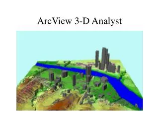
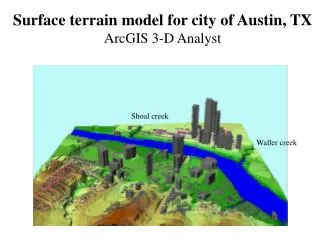
Surface terrain model for city of Austin, TX ArcGIS 3-D Analyst. Shoal creek. Waller creek. Triangulated Irregular Network (TIN) A lgorithm for i nterpolating i rregularly- s paced data in terrain modeling. UT Campus. D igital representation of the terrain

E N D
Surface terrain model for city of Austin, TXArcGIS 3-D Analyst Shoal creek Waller creek
Triangulated Irregular Network (TIN)Algorithm for interpolating irregularly-spaced data in terrain modeling UT Campus
Digital representation of the terrain Preserves details of a shape on the terrain, more accurate representation of urban area Break lines represent significant terrain features like a lake or cliff that cause a change in slope Requires a much smaller number of points than a gridded DTM (The digital terrain model) in order to represent the surface terrain with equal accuracy A triangular mesh is drawn on the control and determined data points A perimeter around the data points is first established, the convex hull To connect the interior points, Delaunay triangulation is used A surface is created by integrating all of the triangles over the domain Additional elevation data such as spot elevations at summits and depressionsand break lines are also collected for the TIN model TIN Steps to Form a Surface From TIN
A Mesh of Triangles in 2-D Triangle is the only polygon that is always planar in 3-D Lines Surfaces Points
TIN Triangles in 3-D (x3, y3, z3) (x1, y1, z1) (x2, y2, z2) z y Projection in (x,y) plane x
Delauney Triangulation • Developed around 1930 to design the triangles efficiently • Geometrically related to theissen tesselations • Maximize the minimum interior angle of triangles that can be formed • No point lies within the circumcircle of a triangle that is contained in mesh Yes More uniform representation of terrain No
Draw the perpendicular bisectors of each edge of the triangle Circumcircle is centered on their intersection point Radial lines from center have equal length Circumcircle of Triangle
Theissen polygon • Associate each point with the area that is associated with that point more closely than any other • Common for getting rainfall • Widely used without GIS
Soft Breaklines Hard Breaklines Mass Points Inputs for Creating a TIN • Mass Points define points anywhere on landscape • Hard breaklines define locations of abrupt surface change (e.g. streams, ridges, road kerbs, building footprints, dams) • Soft breaklines are used to ensure that known z values along a linear feature are maintained in the tin.
TIN with Linear Surface Features Classroom UT Football Stadium Waller Creek City of Austin digitized all the buildings to get emergency vehicles quickly
Input data for this portion Mass Points not inside building Soft Breaklines along the hills Hard Breaklines along the roads
ESRI TIN EngineIntegrated Terrain Model, ARCGIS 9.2 • Creates varying levels of conditions and points to produce pyramid style TINs on the fly • Provides an efficient methodology for working with mass data • Results in a single dataset that can rapidly deploy and visualize TIN based surfaces at multiple scale Courtesy, http://gis.esri.com
TIN Surface Model Waller Creek Street and Bridge
Data Sources to Develop TINs • LIDAR (Light Detection and Ranging; or Laser Imaging Detection and Ranging) • Aerial photogrammetry
LIDAR • An optical remote sensing technology • Masures properties of scattered light to find range and/or other information of a distant target • LIDAR sensor was mounted on-board • During the flight, the LIDAR sensor pulses a narrow, high frequency laser pulse toward the earth through a port opening in the bottom of the aircraft's fuselage • The LIDAR sensor records the time difference between the emission of the laser beam and the return of the reflected laser signal to the aircraft • Range to an object is determined by measuring the time delay between transmission of a pulse and detection of the reflected signalto the aircraft • Points are distributed across the space, push-broom sensor • Amazing degrees of details. Resolution is 1/9 arc second • 1 arc second DEM = 30 m • 1/3 arc second DEM = 10 m
EAARL LIDAR Topography of Platte River and Floodplain Near Overton, NE
Aerial photogrammetry • The aerial photos are taken using a stereoscopic camera • Two pictures of a particular area are simultaneously taken, but from slightly different angles, overlapping photographs • The overlapping area of the two resulting photos is called a stereo pair • Using a computer, stereoplotter, the stereo pair can be viewed as a single image with the appearance of depth or relief • Ground control points are established based on ground surveys or aerial triangulation and are viewed in the stereoplotter in conjunction with the stereo pair • The image coordinates of any (x,y,z) point in stereoscopic image paircan be determined and randomly selected and digitized
LIDAR Terrain Surface for Powder River, Wyoming Source: Roberto Gutierrez, UT Bureau of Economic Geology
NCALM National Center for Airborne Laser Mapping • Sponsored by the National Science Foundation (NSF) (http://www.ncalm.org) • Operated jointly by the Department of Civil and Coastal Engineering, College of Engineering, University of Florida (UF) and the Department of Earth and Planetary Science, University of California- Berkeley (UCB) • Invites proposals from graduate students seeking airborne laser swath mapping (ALSM) observations covering limited areas (generally no more than 40 square kilometers) for use in research to earn an M.S. or PhD degree. • Proposals must be submitted on-line by November 30, 2006
Some advantages of TINS • Fewer points are needed to represent the topography---less computer disk space • Points can be concentrated in important areas where the topography is variable and a low density of points can be used in areas where slopes are constant. • Points of known elevation such as surveyed benchmarks can easily be incorporated • Areas of constant elevation such as lakes can easily be incorporated • Lines of slope inflection such as ridgelines and steep canyons streams can be incorporated as breaklines in TINS to force the TIN to reflect these breaks in topography
Why interpolate to raster? Analogy: Spatially distributed objects are spatially correlated; things that are close together tend to have similar characteristics
Interpolation using Rasters • Interpolation in Spatial Analyst • Inverse distance weighting (IDW) • Spline • TOPOGRID, Topo to Raster (creation of hydrologically correct digital elevation models) • Kriging (utilize the statistical properties of the measured points & quantify the spatial autocorrelation among measured points ) • Interpolation in Geostatistical Analyst.
Using the ArcGIS Spatial Analyst to create a surface using IDW interpolation • Each input point has a local influence that diminishes with distance • It weights the points closer to the processing cell greater than those farther away • With a fixed radius, the radius of the circle to find input points is the same for each interpolated cell • By specifying a minimum count, within the fixed radius, at least a minimum number of input points is used in the calculation of each interpolated cell • A higher power puts more emphasis on the nearest points, creating a surface that has more detail but is less smoot • A lower power gives more influence to surrounding points that are farther away, creating a smoother surface. Search is more globally
Using the ArcGIS Spatial Analyst to create a surface using IDW interpolation IDW weights assigned arbitrarily
ArcGIS Spatial Analyst to create a surface using Topo to Raster interpolation • Designed for the creation of hydrologically correct digital elevation models • Interpolates a hydrologically correct surface from point, line, and polygon • Based on the ANUDEM program developed by Michael Hutchinson (1988, 1989) • The ArcGIS 9.x implementation of TopoGrid from ArcInfo Workstation 7.x • The only ArcGIS interpolator designed to work intelligently with contour inputs • Iterative finite difference interpolation technique • It is optimized to have the computational efficiency of local interpolation methods, such as (IDW) without losing the surface continuity of global interpolation methods, such as Kriging and Spline
Using the ArcGIS Spatial Analyst to create a surface using Spline interpolation • Best for generating gently varying surfaces such as elevation, water table heights, or pollution concentrations • Fits a minimum-curvature surface through the input points • Fits a mathematical function to a specified number of nearest input points while passing through the sample points • The REGULARIZED option usually produces smoother surfaces than those created with the TENSION • For the REGULARIZED, higher values used for the Weight parameter produce smoother surfaces • For the TENSION, higher values for the Weight parameter result in somewhat coarser surfaces but with surfaces that closely conform to the control points • The greater the value of Number of Points, the smoother the surface of the output raster
Interpoloation using Kriging • Things that are close to one another are more alike than those farther away : spatial autocorrelation • As the locations get farther away, the measured values will have littlerelationship with the value of the prediction location Kriging weights based on semivariogram
SemiVariagram Captures spatial dependence between samples by plotting semivariance against seperation distance • Sill The height that the semivariogram reaches when it levels off. • Range:The distance at which the semivariogram levels off to the sill • Nugget effect: a discontinuity at the origin (the measurement error and microscale variation )
SemiVariagram h = separation distance between i an j
What information does it provide? • The γ between samples separated by no distance is about 1.5E-4 • Points influence each other within 60 km, beyond that they don’t • An unmeasured location can be predicted based on its neighboring samples closer than 60 km • The points separated by 60 km are likely to have the same average difference as points separated by 100 km or any distance above 60 km
Case Study: Estimating Fecal Coliform Levels in Galveston Bay, TX Observed fecal coliform concentrations for January 1999 (MPN fecal coliform colonies/100ml of water )
Study site characteristics Consists of 5 bay segments 40 Upstream drainage area 5 managed water quality segments Each treated differently in TX High Concentration of bacteria in Urban Concentration is low away from urban Major area of contamination is associated with Huston (4 106) Industrial sources (refinery) Bacteria tend to be local because they die off pretty past
Exploratory Spatial Data Analysisin Geostatistical Analysis • Histogram • Normal Q-Q (Quantile-Quantile) plot • Trend Analysis • Voronoi Map • Semivariogram Cloud • General Q-Q Plot • Crosscovariance Cloud
2. Normal Q-Q plot Standard normal distribution Log of bacteria conc.
2. Normal Q-Q plot Standard normal distribution Log of bacteria conc. Samples with no detection of bacteria Mean bacteria C = 1.59 log units ~40 Decision Criteria for Environmental Management Task: % of data exceed certain threshold (43) Samples with no detection of bacteria conc. =2
3. Trend Analysis • 3D plot of the samples and a regression on the attribute in the XZ and YZ planes • Visualize the data and to observe any large-scale trends that the modeler might want to remove prior to estimation
Cross Validation of the Model • Uses all of the data to estimate the trend and autocorrelation models • It removes each data location, one at a time, and predicts the associated data value. • For example, the diagram below shows 10 randomly distributed data points. Cross Validation omits red point and calculates the value of this location using the remaining blue points • The predicted and actual values at the location of the omitted point are compared • This procedure is repeated for a second point, and so on • For all points, cross-validation compares the measured and predicted values