Modeling and Solving LP Problems in a Spreadsheet
Chapter 3. Modeling and Solving LP Problems in a Spreadsheet. Introduction. Solving LP problems graphically is only possible when there are two decision variables Few real-world LP have only two decision variables Fortunately, we can now use spreadsheets to solve LP problems.

Modeling and Solving LP Problems in a Spreadsheet
E N D
Presentation Transcript
Chapter 3 Modeling and Solving LP Problems in a Spreadsheet
Introduction • Solving LP problems graphically is only possible when there are two decision variables • Few real-world LP have only two decision variables • Fortunately, we can now use spreadsheets to solve LP problems
Spreadsheet Solvers • The company that makes the Solver in Excel, Lotus 1-2-3, and Quattro Pro is Frontline Systems, Inc. Check out their web site: http://www.solver.com • Other packages for solving MP problems: AMPL LINDO CPLEX MPSX
Preparation: Install Premium Solver • You must have a PC, not a MacIntosh. If you have a MacIntosh, plan to work in the computer lab Zone 1. • Quit from Excel • Execute PremSolv.exe
Preparation: the Model • Make sure you have a model, written in correct form. • We’ll use the example from your textbook.
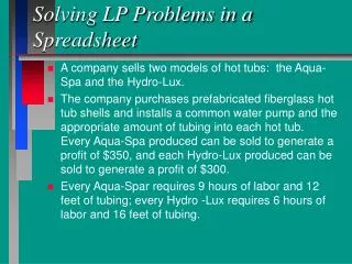
Preparation: the Model Blue Ridge Hot Tubs MAX Z = 350X1 + 300X2} profit Subject to: 1X1 + 1X2 <= 200 } pumps 9X1 + 6X2 <= 1566 } labor 12X1 + 16X2 <= 2880 } tubing Legend: X1 = Number of Aquaspas to make X2 = Number of Hydroluxes to make
Entering the model in ExcelStep 1: Give your model a cool title
Step 2: Set up the columns II. Add one column for each unknown in the legend Legend: X1 = Number of Aquaspas to make X2 = Number of Hydroluxes to make III. Reserve a column on the right side for all the spreadsheet formulas I. Reserve the 1st column for row labels IV. Add a label for what you are trying to Maximize or to Minimize
Step 3: Enter the objective function Legend: X1 = Number of Aquaspas to make X2 = Number of Hydroluxes to make MAX Z = 350X1 + 300X2 } profit I. Unknowns will go in the first row. Enter 0 in these cells, since we don’t know what they’ll be. III. In the row underneath the unknowns, put the coefficients. IV. Enter a nice explanatory label for the objective function coefficients II. Refer to the legend and add a nice explanatory label for the row of unknowns
Step 3: Enter the objective function, cont. Legend: X1 = Number of Aquaspas to make X2 = Number of Hydroluxes to make MAX Z = 350X1 + 300X2 } profit V. Enter a formula for the objective function, multiplying each coefficient cell by the unknown in the cell above it. Add each pair together.
Step 4: Add pretty colors I. Use the font color icon to add color, improving readability II. Use the cell shading icon to add background shading, improving readability
Step 6: Enter the constraints Legend: X1 = Number of Aquaspas to make X2 = Number of Hydroluxes to make 1X1 + 1X2 <= 200 } pumps 9X1 + 6X2 <= 1566 } labor 12X1 + 16X2 <= 2880 } tubing II. List the constraints I. Insert a label to show where the constraints are located
Step 6: Enter the constraints, cont. Legend: X1 = Number of Aquaspas to make X2 = Number of Hydroluxes to make III. Enter the constraint coefficients. 1X1 + 1X2 <= 200 } pumps 9X1 + 6X2 <= 1566 } labor 12X1 + 16X2 <= 2880 } tubing IV. Skip a column and enter the right-hand side values.
Step 6: Enter the constraints, cont. Legend: X1 = Number of Aquaspas to make X2 = Number of Hydroluxes to make 1X1 + 1X2 <= 200 } pumps 9X1 + 6X2 <= 1566 } labor 12X1 + 16X2 <= 2880 } tubing Enter formulas for the constraints, multiplying each constraint coefficient times the unknown above it.
Running Solver • With the spreadsheet now set up, it’s time to run the Solver utility.
Running Solver Step 1 • Select Tools..Add-ins and make sure the Solver Add-in is checked. (Click on thecheck box if it isn’t.) • Click OK • If the Solver Add-In is not showing at all, plan on working in the lab Zone 1.
Running solver: Step 1 cont. • Select the Tools..Solver menu item • If the Standard Solver window appears, click the Premium button
Running Solver Step 1 cont. I. Click the options button II. When the Solver Options window appears, make sure Assume Linear Model and Assume Non-Negative are both checked. III. Click OK.
Running Solver: Step 2 • In the Premium Solver window, set the solution method to Standard Simplex LP
How Solver Views the Model Constraint cells - the cells in the spreadsheet representing the constraint formulas the constraint right-hand sides Changing cells - the cells in the spreadsheet representing the decision variables Set Cell - the cell in the spreadsheet that represents the objective function
Running Solver: Step 3 Click in the Set Cell textbox, then click the cell in the spreadsheet. The appropriate cell reference will appear in the textbox.
Running Solver: Step 4 Click in the Changing Variable Cells textbox, then click and drag the spreadsheet cursor to highlight all the unknowns in the objective functions. The appropriate cell references will appear in the textbox.
Running Solver: Step 5 I. Click the Add button. II. The Add Constraint dialog box appears. III. Click in the Cell Reference textbox, then click the cell with the constraint formula. IV. Click in the Constraint textbox, then click on righthand side value for the constraint. V. Set inequality. VI. Click the OK button.
Running Solver: Step 6 Add all remaining ineqalities
Running Solver: Step 7 I. Click solve II. Check to see if solver found a solution. III. If solver did not find a solution, click OK. IV. Look for errors in the solver parameters and try again.
Running Solver: Step 7 cont. I. If solver found a solution II. Highlight all three reports by clicking on them. III. Click OK to close window. IV. Click Close to close window.
Running Solver: Step 7 cont. V. Various linear programming reports will have been added to the spreadsheet. V. Click on Answer Report to view the solution.
Instructor opinion • You can set up the spreadsheet differently, but for beginners it’s best to use the same spreadsheet design. • Once you can get it to work the way described in this handout/powerpoint, feel free to try other approaches. • Let’s do another.
Model 1 Model 2 Model 3 Number ordered 3,000 2,000 900 Hours of wiring/unit 2 1.5 3 Hours of harnessing/unit 1 2 1 Cost to Make $50 $83 $130 Cost to Buy $61 $97 $145 Make vs. Buy Decisions:The Electro-Poly Corporation • Electro-Poly is a leading maker of slip-rings. • A $750,000 order has just been received. • The company has 10,000 hours of wiring capacity and 5,000 hours of harnessing capacity.
Convert to model Minimize the total cost of filling the order. MIN: 50M1+ 83M2+ 130M3+ 61B1+ 97B2+ 145B3 Legend: M1 = Number of model 1 slip rings to make in-house M2 = Number of model 2 slip rings to make in-house M3 = Number of model 3 slip rings to make in-house B1 = Number of model 1 slip rings to buy from competitor B2 = Number of model 2 slip rings to buy from competitor B3 = Number of model 3 slip rings to buy from competitor • Demand Constraints • M1 + B1 = 3,000 } model 1 • M2 + B2 = 2,000 } model 2 • M3 + B3 = 900 } model 3 • Resource Constraints • 2M1 + 1.5M2 + 3M3 <= 10,000 } wiring • 1M1 + 2.0M2 + 1M3 <= 5,000 } harness
Years to Company Return Maturity Rating Acme Chemical 8.65% 11 1-Excellent DynaStar 9.50% 10 3-Good Eagle Vision 10.00% 6 4-Fair Micro Modeling 8.75% 10 1-Excellent OptiPro 9.25% 7 3-Good Sabre Systems 9.00% 13 2-Very Good An Investment Problem:Retirement Planning Services, Inc. • A client wishes to invest $750,000 in the following bonds.
Investment Restrictions • No more than 25% can be invested in any single company. • At least 50% should be invested in long-term bonds (maturing in 10+ years). • No more than 35% can be invested in DynaStar, Eagle Vision, and OptiPro.
Defining the Decision Variables X1 = amount of money to invest in Acme Chemical X2 = amount of money to invest in DynaStar X3 = amount of money to invest in Eagle Vision X4 = amount of money to invest in MicroModeling X5 = amount of money to invest in OptiPro X6 = amount of money to invest in Sabre Systems
Defining the Objective Function Maximize the total annual investment return: MAX: .0865X1+ .095X2+ .10X3+ .0875X4+ .0925X5+ .09X6
Defining the Constraints • Total amount is invested X1 + X2 + X3 + X4 + X5 + X6 = 750,000 • No more than 25% in any one investment Xi <= 187,500, for all i • 50% long term investment restriction. X1 + X2 + X4 + X6 >= 375,000 • 35% Restriction on DynaStar, Eagle Vision, and OptiPro. X2 + X3 + X5 <= 262,500 • Nonnegativity conditions Xi >= 0 for all i
Implementing the Model See file Fig3-20.xls
Processing Plants Groves Distances (in miles) Supply Capacity 21 Mt. Dora Ocala 200,000 275,000 1 4 50 40 35 30 Eustis Orlando 600,000 400,000 2 5 22 55 20 Clermont Leesburg 225,000 300,000 3 6 25 A Transportation Problem: Tropicsun
Defining the Decision Variables Xij= # of bushels shipped from node ito node j Specifically, the nine decision variables are: X14 = # of bushels shipped from Mt. Dora (node 1) to Ocala (node 4) X15 = # of bushels shipped from Mt. Dora (node 1) to Orlando (node 5) X16 = # of bushels shipped from Mt. Dora (node 1) to Leesburg (node 6) X24 = # of bushels shipped from Eustis (node 2) to Ocala (node 4) X25 = # of bushels shipped from Eustis (node 2) to Orlando (node 5) X26 = # of bushels shipped from Eustis (node 2) to Leesburg (node 6) X34 = # of bushels shipped from Clermont (node 3) to Ocala (node 4) X35 = # of bushels shipped from Clermont (node 3) to Orlando (node 5) X36 = # of bushels shipped from Clermont (node 3) to Leesburg (node 6)
Defining the Objective Function Minimize the total number of bushel-miles. MIN: 21X14 + 50X15 + 40X16 + 35X24 + 30X25 + 22X26 + 55X34 + 20X35 + 25X36
Defining the Constraints • Capacity constraints X14 + X24 + X34 <= 200,000 } Ocala X15 + X25 + X35 <= 600,000 } Orlando X16 + X26 + X36 <= 225,000 } Leesburg • Supply constraints X14 + X15 + X16 = 275,000 } Mt. Dora X24 + X25 + X26 = 400,000 } Eustis X34 + X35 + X36 = 300,000 } Clermont • Nonnegativity conditions Xij>= 0 for all iandj
Implementing the Model See file Fig3-24.xls
Percent of Nutrient in Nutrient Feed 1 Feed 2 Feed 3 Feed 4 Corn 30% 5% 20% 10% Grain 10% 3% 15% 10% Minerals 20% 20% 20% 30% Cost per pound $0.25 $0.30 $0.32 $0.15 A Blending Problem:The Agri-Pro Company • Agri-Pro has received an order for 8,000 pounds of chicken feed to be mixed from the following feeds. • The order must contain at least 20% corn, 15% grain, and 15% minerals.
Defining the Decision Variables X1 = pounds of feed 1 to use in the mix X2 = pounds of feed 2 to use in the mix X3 = pounds of feed 3 to use in the mix X4 = pounds of feed 4 to use in the mix
Defining the Objective Function Minimize the total cost of filling the order. MIN: 0.25X1 + 0.30X2 + 0.32X3 + 0.15X4
Defining the Constraints • Produce 8,000 pounds of feed X1 + X2 + X3 + X4 = 8,000 • Mix consists of at least 20% corn (0.3X1 + 0.5X2 + 0.2X3 + 0.1X4)/8000 >= 0.2 • Mix consists of at least 15% grain (0.1X1 + 0.3X2 + 0.15X3 + 0.1X4)/8000 >= 0.15 • Mix consists of at least 15% minerals (0.2X1 + 0.2X2 + 0.2X3 + 0.3X4)/8000 >= 0.15 • Nonnegativity conditions X1, X2, X3, X4 >= 0
A Comment About Scaling • Notice the coefficient for X2 in the ‘corn’ constraint is 0.05/8000 = 0.00000625 • As Solver runs, intermediate calculations are made that make coefficients larger or smaller. • Storage problems may force the computer to use approximations of the actual numbers. • Such ‘scaling’ problems sometimes prevents Solver from being able to solve the problem accurately. • Most problems can be formulated in a way to minimize scaling errors...
Re-Defining the Decision Variables X1 = thousands of pounds of feed 1 to use in the mix X2 = thousands of pounds of feed 2 to use in the mix X3 = thousands of pounds of feed 3 to use in the mix X4 = thousands of pounds of feed 4 to use in the mix
Re-Defining the Objective Function Minimize the total cost of filling the order. MIN: 250X1 + 300X2 + 320X3 + 150X4