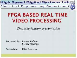
FPGA BASED REAL TIME VIDEO PROCESSING
FPGA BASED REAL TIME VIDEO PROCESSING . Final B presentation Duration : year. Presented by: Roman Kofman Sergey Kleyman Supervisor: Mike Sumszyk . AGENDA. Project Objectives. AGENDA. Algorithm - review. Based on the 2D non-linear Diffusion equation Iterative solution

FPGA BASED REAL TIME VIDEO PROCESSING
E N D
Presentation Transcript
FPGA BASED REAL TIME VIDEO PROCESSING Final B presentation Duration : year Presented by: Roman Kofman Sergey Kleyman Supervisor: Mike Sumszyk
Algorithm - review • Based on the 2D non-linear Diffusion equation • Iterative solution • Good Filtering – smoothes noises • Keeps borders intact
Matlab simulation Filtered image Original image
Thomas Consists of three loops – one of which is reversed β,m,y are vectors of length N (frame resolution) and need to be stored in memory since they are read backwards The original Thomas requires memory of at least four times the frame size. α(1) β(1) 0 0 … γ(1) α(2) β(2) 0 … 0 γ(2) α(3) β(3) … .. … … β(N-1) 0 0 0 γ(N-1) α(N) for i=1:N-1 l(i) = gamma(i)/m(i); m(i+1) = alpha(i+1)-l(i)*beta(i); end y=u; y(1)=d(1); for i=2:N y(i)=d(i)-l(i-1)*y(i-1); end u(N)=y(N)/m(N); for i=N-1:-1:1 u(i)=(y(i)-beta(i)*u(i+1))/m(i); end
Memory efficient implementation • The inverse of a block diagonal matrix is another block diagonal matrix, composed of the inverse of each block • We flip each row separately, this way internal memory would be sufficient • Requires selective treatment of borders
Error criteria We use the relative Root Mean Square Error as an error criteria. The RRMSE2 is defined by: Where: XA is the filtered image XR is the relative image
Fixed point considerations Matlab simulations showed that during calculations we need to work with 16bits: Original image Full precision Fixed point RMSE=0.0416 dt=5, 4 iterations
Data Flow - One Iteration Two parallel channels Columns T’ T’ M4K LINE REVERSE READ M4K LINE REVERSE READ M4K LINE REVERSE READ M4K LINE REVERSE READ • M4K LINE REVERSE WRITE • M4K LINE REVERSE WRITE • M4K LINE REVERSE WRITE • M4K LINE REVERSE WRITE DVI IN DVI OUT How to implement T’ In real time? Lines PIPE PIPE Thomas 3 Thomas 3
Project B - “divide and conquer” Divide between 2 problems: Algorithm and Memory access • Implement algorithm on a small frame – our part • Complete implementation of transpose using DDR – Neta and Hillel • Integrate both parts into one full data path
Project B motivation and goals • Implement the algorithm in a scalable manner • Display results for a small frame • Implement the transpose in internal memory • Implement blocks that will create the mini frame at the beginning and generate full frame at the end DVI IN Algorithm DVI OUT Create mini frame Generate large frame
Mini from full: using internal memory we select a small frame, and send it in a burst to the pipe • As to fit the internal memory of the FPGA, we choose a 100*100 mini frame • The implementation of the algorithm is scalable to larger frames • Full out of mini: after the algorithm we generate large frame by zero padding the mini frame
Data path for mini frame processing Thomas loop 1 Thomas loop 2 Thomas loop 3 MRamTriPort M4K Row flip on M4K Mram TriPort control control control control Sync signals Sync signals Sync signals Upscalable to full frame processing Normal and transpose read of mini frame Pipeline Row flip Pipeline Row flip Full frame generation
Synchronization signals • As mentioned, we must treat borders differently then normal pixels. • Therefore – we must distinguish throughout the entire pipeline between borders and non borders, and whether it is start or end. • To do so – we generate four sync signals, that describe every pixel Start of column Start of line End of line End of column
The need for these signals had upraised in the algorithm, but we can now use these signals for memory sync and frame generation sync From the four signals we can easily derive a “start frame” signal, and also an “end frame” signal.
Transpose in internal memory • Transpose the image during reading • read address is a sum of two weighted values: row and column pointers • Transpose the image by switching the pointers Column pointer weight Row pointer Transposed read address Row pointer weight Column pointer Normal read address
Row flip on internal memory • Use M4K memory to reverse order on incoming data for entire row • Implement scalable design to be used on different row sizes • Use sync signals as inputs and generate them for the next block at the output
From Matlab to HDL - Simulink phase • From serial code to a combination of sequential and parallel blocks • “Close to hardware” implementation • Real time simulation and comparison to code (non real time) results
Simulation in Simulink • Data from DVI • Using repeating sequence block • Emulating Row flip • Using enabled system for sync • Buffer depth is number of pixels in a row
Simulink data path Derivatives calculation Thomas forward loops Double buffered flip – memory emulation Thomas reversed loop Double buffered flip – memory emulation Building tri-diagonal matrix
From Matlab to HDL – SinplifyDSP phase • From full precision Simulink blocks, to fixed point hardware representing blocks • Pipelining and frequency considerations • Generate HDL code
From Matlab to HDL – SinplifyDSP phase • After transforming every part of the data path from Simulink blocks to SinplifyDSP blocks and synthesizing– not all parts achieved the required frequency (DVI clk ~25MHz) • The critical paths were in the loops in the design – unfortunately you can’t pipeline a loop • Solution: Simplify every loop as much as possible
Simplifying loops – Thomas 1 Loops with heavy calculations become critical paths Move multiplier out of loop Pipeline
Simplifying loops • After movements – the maximum frequency is still to low • Solution: Replace the SinplifyDSP division block with faster but less accurate implementation – AEPG division algorithm
Anderson, Earle, Goldschmidt and Powers division algorithm • Iterative algorithm that calculates N/D • Adding iterations increases precision but uses more resources (extra multipliers and sums)
Simplifying loops – Thomas 2 • The change in Thomas 1 influenced Thomas 2
Integrating the Sinplify projects into one Quartus project • SinplifyDSP generates registers and blocks with default similar names • Simple combine in Quartus will not work • Combining several blocks in Quartus demands different approach • Manually change names – not realistic as to the huge amount of blocks • Combine all the Sinplify projects to one and use black boxes to include VHDL code for the row flip – works, but synthesize is very long (could be days) • Use design partitions – our recommended method – dramatically shortens synthesizes and allows simple modular design !
Functional and timing simulations • Using the design partitions method – we created test benches to test every block in Modelsim - functional simulation • After correct functional simulation in Modelsim, we repeated this simulation in Quartus simulator tool • We then did a timing simulation in the simulator tool
Functional and timing simulations Algorithm Mini frame related • Tested the Simulink phase in comparison with theoretic matlab code • Tested the SinplifyDSP phase in comparison with theoretic matlabcode and tested synchronization • Tested in Modelsim for functional operation • Tested timing in Quartus • View real time results on screen • Tested in Modelsim for functional operation • Tested timing in Quartus • View real time results on screen
Results • Algorithm works correctly and gives correct results –ready to be upscaled • For large dt values we get artifacts – also seen in Matlab fixed point simulations • Unresolved sync problem in the mini frame creation – only a problem for displaying the mini frame
Upscaling to a full frame • Change parameters in SinplifyDSP(N_col, N_row), Synthesize and create design partitions • Change memory size for the row flip • Change parameters throughout the design (Generic parameters) • Remove mini from full and full from mini, and integrate with Neta’s and Hillel’s data path • Synthesize, place and route in Quartus
Achievements • Algorithm and pipeline working at ~26MHz (a bit higher then DVI clk) • One iteration is enough to see results. Maximum stable dt is ~5 (In comparison to semi implicit design where dt was only limited to 0.5) • Display real time results and improve video quality • Unfortunately, Still having some unresolved problems with sync
Insights and conclusions • Signal processing in real time is quite hard and demands precise planning and designing • Test benches must be used to test every part of the design • The principle of “divide and conquer” is a gateway to success • You should be familiar with the available tools prior to beginning working • Documentation is, unfortunately, not complete and sometimes not accurate • Compatibility, versions and lack of remote access
Thank you for listening… We invite you to join us in the lab for a short demonstration