Segmentation, contour based
Segmentation, contour based. A segmented image contains groupings of parts of an image that are homogenous in one or more properties: intensity or color texture (the fine structure in intensity) movement (a vector value per pixel).

Segmentation, contour based
E N D
Presentation Transcript
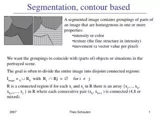
Segmentation, contour based • A segmented image contains groupings of parts of an image that are homogenous in one or more properties: • intensity or color • texture (the fine structure in intensity) • movement (a vector value per pixel) We want the groupings to coincide with (parts of) objects or situations in the portrayed scene. The goal is often to divide the entire image into disjoint connected regions: Image = k Rk with RiRj = for i j R is a connected region if for each xi and xj in R there is an array {xi,..., xk, xk+1,..., xj } in R where each consecutive pair (xk, xk+1 ) is connected (4,8 or mixed). Theo Schouten
Boundary and regions • We can try to find both the boundaries of the regions and the regions themselves. • Perfect boundaries and regions are redundant, from one you can derive the other • The methods for finding them differ largely in character and suitability for application in particular concrete cases. • Boundary- and area-finding techniques can be combined (hybrid segmentation) to yield a more reliable segmented image. • In this chapter "knowledge" becomes important. This can be defined as implicit or explicit limits to the probability of a given grouping in an image. • This knowledge can be domain dependent, for example: • this is an image of blocks • there is an airplane to the top left, etc. • It can also be general, physical or heuristical knowledge • most humans have two arms • the maximum velocity or acceleration with movement • preference for the shortest edge between two points Theo Schouten
Edges Edges of objects are important for the human visual system, often objects can already be recognized by simply a rough contour. It is difficult to detect the contours of objects directly from an intensity image. It's a better idea to first convert the image to one that shows local discontinuities (edges) in the intensity. An edge is a vector that shows a particular position, size and direction of a discontinuity. Sometimes only the size is determined. The "direction" of the edge is perpendicular to the "direction" of the contour of the object, pay close attention to the directions used. An edge can be determined per pixel, but also between connected pixels, the so-called crack edges. Sometimes the position of an edge is determined with a higher precision than one pixel. Theo Schouten
Edge operator • An edge operator is a mathematical function that detects local discontinuities in a limited space. • The edge operators can be classified into: • approximation of the gradient operator • template matching, check if edge-models fit • fit with parameterized edge-models, when more is known about the edges which one wants to find. • All edge operators have a certain underlying model about the discontinuities which they detect. • They yield numbers for the size and direction of the discontinuities, independent of how well that local image piece satisfies the model. • This quality of the "match" is often hidden in the size, but sometimes also in separated quality or threshold values. Theo Schouten
Parameterized edge model operators These operators cost a lot of calculation time and their benefit is fairly limited; especially as a general edge operator, which can be used without a lot of a priori information about the image scene. They can yield more information about the discontinuity than direction and size alone, such as the width of an edge and the size of intensity transitions to the left and right of the image. Theo Schouten
Points and lines Isolated pixels are often detected with masks that approximate the Laplacian. These operations are very sensitive to noise. Thresholding yields the pixels that drastically deviate from their neighborhood. Lines that are one pixel broad can be found using the masks below. Select direction i if: |Ri| > |Rj| for all j, possibly (weighted with |Rk|) averaging values when two directions close to each other yield almost the same R. Thresholding (absolute and relative) is used to remove non-relevant line-elements. Theo Schouten
Gradient Using the image function f(x,y) one can determine the vector gradient image: f(x,y) = ( f/x, f/y ) = arctan2( f/x , f/ y ) direction ( ( f/x)2 + (f/y)2 ) size | f/x| + | f/y| often used as approximation f/x = f(x+1,y) - f(x,y) , f/y = f(x,y +1) - f(x,y) “crack” edges Theo Schouten
Roberts, Prewitt, Sobel masks Prewitt and Sobel take more pixels into account and are thereby less sensitive to noise. Variants with 2 are also used a lot. Larger masks, for example 5 by 5, can be used, if by approximation the edges are straight over such a large area. Theo Schouten
Example Sobel Original edge size, 3x3 Sobel x and y components of Sobel Theo Schouten
Laplacian example Landsat image (channel 5) 4-connected Laplacian Part Laplacian with zero- crossing Theo Schouten
Laplacian of Gaussian (LoG) Marr and Hildreth used the Laplacian of Gaussian function: h(x,y) = exp( - (x2+y2) / 2 2 )2 h(r) = ( (r2- 2) / 2) exp(-r2 / 2 2) the "mexican hat" function, and determined the convolution of it with an image. This is the same as first determining the convolution of the image with the Gaussian (=smoothing) and then taking the Laplacian of it. The convolution matrices are large ( 9x9 for = 1, 43x43 for = 5), but the calculations can be made faster because the LoG is separable: LoG(x,y) = h12(x,y) + h21(x,y) with h12(x,y) = h1(x)h2(y) and h21(x,y) =h2(x)h1(y). The LoG can also be approximated with a DoG ( Difference of Gaussian’s with different ’s). There are indications that biological systems also do this. Theo Schouten
Example LoG Original image Sobel gradient Gaussian smoothing Laplacian LoG thresholded LoG zero-crossings Theo Schouten
Canny Canny (1986) uses a first order derivative. Starting with a 1-D step edge around 0 with white Gaussian noise and a convolution with an antisymmetric function I(x), the following maxima yield the 1-D edges: (x0) = - +I(x) f(x-x0) dx • He first determined the best I(x) for efficient edge detection assuming certain criteria and expressed them as mathematical functions: • good detection: small chance of missing real edges and finding false ones. • good localization: small difference found-real edges • just one position per edge • His best I(x) can be approximated (20% worse) by the first derivative of a Gaussian: • (x / 2) exp( -x2 / 2) Theo Schouten
Canny 2D In 2-D we want to execute a convolution with the first derivative of a 2-D Gaussian in a direction n perpendicular to the edge: Gn = G/ n = n . G with G = (G/x, G/ y)n = (G Im) / | (G Im) | (this is true for approximation) ( GnIm) / n = 0 thus 2 (G Im) / n2 = 0 (local maximum) In his implementation Canny used simple masks to calculate n and a simple peak-determination with one threshold in the direction of n. There now exists better methods to axproximate this. Deriche (1987) found an I(x) that was 90% better than the derivative of the Gaussian and can also be implemented rapidly. In 2-D the derivatives can be found by convolution with masks that are separable (13 * and 12 + per pixel). Theo Schouten
Example Canny Landsat image Canny edges Edge directions after thinning Theo Schouten
Templates Often motivated by the Kirsch operator: S(x) = maxkk-1k+1 |f(xk)-f(x)| (x) = kmax * 45° k walks around x : 4 3 2 5 x 1 6 7 8 Possible implementation: |-3 -3 5| |-3 5 5| | 5 5 5| |-3 -3 -3||-3 5| |-3 5| |-3 -3| ... |- 3 5||-3 -3 5| |-3 -3 -3| |-3 -3 -3| |-3 5 5| This uses 8 templates, so 8 values are calculated for each pixel in the image. The template with the highest value defines the edge strength (equal to that value) and the edge direction (quantized in steps of 45°). Edges with a small magnitude are often caused by noise or small fluctuations. Thresholding is then used to remove weak edges: S'(x) = 0 if S(x) Threshold otherwise S(x) Theo Schouten
Frei and Chen The image function around point x0 is factorized as a sum over 9 basis functions: f(x) = k=08 (f, hk) hk(x- x0 ) / (hk, hk) around x0 with (f, hk) = d f(x) hk (x- x0 ) Frei and Chen took the following basis functions: |1 1 1| |-1 -2 -1| | 0 -1 2| | 0 1 0| | 1 -2 1| |1 1 1| | 0 0 0| | 1 0 -1| |-1 0 1| |-2 4 -2| |1 1 1| | 1 2 1| |-2 1 0| | 0 -1 0| | 1 -2 1| |-1 0 1| | 2 -1 0| |-1 0 1| |-2 1 -2| |-2 0 2| |-1 0 1| | 0 0 0| | 1 4 1| |-1 0 1| | 0 1 -2| | 1 0 -1| |-2 1 -2|nostructure gradient ripple line point Every basis function corresponds to a certain local shape in the image, the corresponding coefficient indicates the strength of it. Theo Schouten
Frei and Chen, thresholding How much the image around x0 looks like an edge is then determined as E= k=12 (f, hk)2 and compared with how much it looks like a non-edge (uniform + ripple + line + point): NE = k !=1,2 (f, hk)2. The Frei-Chen threshold then becomes a corner in the NonEdge - Edge space instead of only a threshold value in the Edge direction. Another way of removing noise and double edges is: S'(x) = S(x) if S(x) is a local maximum, else 0 To determine a local maximum one can look at the 4-connected or 8-connected neighboring pixels. Theo Schouten
Edge thinning A simple way of thinning is comparing the pixel strength in the gradient direction (perpendicular to the edge) of each edge pixel to its neighboring pixels. An edge not having the maximal strength is removed. Problems often arise when boundaries come together: (î : an arrow pointing upwards, /: arrow pointing to the top right)) pixels direction magnitude thinned edges 0 0 0 0 0 0 0 0 0 0 0 0 0 0 î î î î î 5 4 3 3 3 0 0 0 + + 2 2 1 1 1 1 1 î î î î î 6 5 4 3 3 + + + + + 2 2 2 1 1 1 1 / / î î / 1 3 3 2 1 0 0 0 0 0 2 2 2 2 2 1 1 / î î î 0 1 2 3 3 0 0 0 + + 2 2 2 2 2 2 2 î î 0 0 0 1 2 0 0 0 0 0 2 2 2 2 2 2 2 Theo Schouten
Lacroix LBE thinnng Lacroix (1988) determines a LBE (likelihood of being a edge) per pixel. Every pixel has two counters: v (visited) and m (maximum). While scanning the image a 3x1 window is placed over every pixel in the gradient direction. Every pixel in the window gets the value v incremented by 1, only the pixel(s) with the highest value get the value m incremented by 1. After the scan LBE becomes LBE = m / v : v m LBE2 2 2 2 2 0 0 0 2 2 0 0 0 1 11 2 3 2 1 1 2 3 2 1 1 1 1 1 12 2 4 3 3 0 0 2 0 0 0 0 1/2 0 01 1 2 4 2 0 0 0 4 2 0 0 0 1 11 0 1 2 2 0 0 0 0 0 0 0 0 0 0 LBEs of 0 are obviously not edges, so LBEs of 1 are then used to start following new contours and lower LBEs are only used to continue with already existing contours. Naturally, during contour-following, different thresholds can be applied to the edge strength. Theo Schouten
Edge relaxation An iterative method to improve edge values by adjusting them depending on the measured edges in the neighborhood. The confidence we have in detecting an edge becomes dependent on the strengths of the edges in the neighborhood: 0 Initial confidence C0(e) e.g.: magnitude / maximal magnitude.1 k=12 for each edge, use the confidences of the neighborhood edges to calculate a type.3 calculate Ck(e)= function { type, Ck-1(e) }4 evaluate convergency criteria (e.g. all the confidences are near to 0 or 1, or the maximal number of iterations has been reached); stop or ( k++ ) and go back to 2. Type=(strong edges left, strong edges right) Ck(e) = Ck-1(e) + C for type (1,1) (1,2) (1,3) and reversibly Ck-1(e) - C for type (0,0) (0,2) (0,3) and reversibly Ck-1(e) all other cases Theo Schouten
Edge linking Edges of neighboring pixels can be combined if they appear similar: | f(x,y) - f(x',y') | < T | (x,y) - (x',y') | < A The first or last edge of each contour can be viewed, possibly taking an average and and adjusting the thresholds to what one already knows about the contour. Can be adapted to detect circles. Theo Schouten
Graph methods Construct a graph from edge values and directions. Use graph algorithms to link edges to contours. Example of a noisy chromosone silhouette determined by graph search. Theo Schouten
Hough transform Look at all the possible lines which can go through an image point (s,t): t = m s + c. The parameters of all these lines form a straight line in the parameter space m,c. Both m and c can attain any value from - to + , what gives problems. In this aspect, a better way to parameterize the line is: x cos + y sin = rThe 's : from -90° to +90° and r: ± 1/2 D , where D is the diagonal of the image. We have the following Hough algorithm to determine lines: - initialize A(rd, d)=0 for all rd and d (make the accumulator matrix discrete) - for every point (x,y) having a value > Threshold : calculate the r’s and ’s for all the possible lines through (x,y), discrete the values to rd and d, then set A(rd, d) := A(rd, d) + 1 for all rd and d - the local maximum in A yields the parameters of lines where a lot of points lie on. Theo Schouten
Hough on points Theo Schouten
Hough on edges For every point (x,y) with edge G(x,y) > Threshold and angle : m = tg ( - /2 ) and c = y - m x Angle is not exact: take a range, e.g. 45 same for x,y: e.g. 1 Theo Schouten
Hough transform for circles Circular figures: x = a + r cos y = b + r sin A static r belongs to a 2-D parameter space A(a,b), a variable r belongs to a 3-D parameter space A(a,b,r). If we want to find both light and dark circles, two sides of every edge must be viewed. If we look at two edges in an image then the number of possible (a,b,r) values strongly decrease. The local maximums in the parameter space are then easier to find. With n edge points (stronger than the threshold) in the image, there are n(n-1)/2 pairs to be viewed. Boundaries on r and testing on the ’s can restrict the number of (a,b,r) values to be calculated.In general, any work done in the parameter space (calculating and tracking down the local maximums) can be replaced by work in the image space. Over the last years the Hough methods have been of much interest because of the development of efficient data structures to save fairly empty A matrixes and to find the local maximums in it. Theo Schouten