COE 405 Combinational Circuit Design
COE 405 Combinational Circuit Design. Dr. Aiman H. El-Maleh Computer Engineering Department King Fahd University of Petroleum & Minerals. Outline. Definitions Boolean Expansion Based on Orthonormal Basis Sum of Product (SOP) Simplification Procedure Don’t Care Conditions

COE 405 Combinational Circuit Design
E N D
Presentation Transcript
COE 405Combinational Circuit Design Dr. Aiman H. El-Maleh Computer Engineering Department King Fahd University of Petroleum & Minerals
Outline • Definitions • Boolean Expansion Based on Orthonormal Basis • Sum of Product (SOP) Simplification Procedure • Don’t Care Conditions • SOP Simplification Procedure using Don’t Cares • Product of Sum (POS) Simplification • Combinational Circuits Design Procedure • Iterative Arithmetic Combinational Circuits • Decoders • Multiplexers
Definitions • A product term of a function is said to be an implicant. • A Prime Implicant (PI) is a product term obtained by combining the maximum possible number of adjacent 1-squares in the map. • A Prime Implicant is a product that we cannot remove any of its literals. • If a minterm is covered only by one prime implicant then this prime implicant is said to be an Essential Prime Implicant (EPI).
Definitions • A cover of a Boolean function is a set of implicants that covers its minterms. • Minimum cover • Cover of the function with minimum number of implicants. • Global optimum. • Minimal cover or irredundant cover • Cover of the function that is not a proper superset of another cover. • No implicant can be dropped. • Local optimum.
Definitions • Let f(x1,x2,…,xn) be a Boolean function of n variables. • The cofactor of f(x1,x2,…,xi,…,xn) with respect to variable xi is fxi = f(x1,x2,…,xi=1,…,xn) • The cofactor of f(x1,x2,…,xi,…,xn) with respect to variable xi’ is fxi’ = f(x1,x2,…,xi=0,…,xn) • Theorem: Shannon's Expansion • Any function can be expressed as sum of products (product of sums) of n literals, minterms (maxterms), by recursive expansion.
Definitions • Example: f = ab + ac + bc • fa = b + c • fa’ = bc • F = a fa + a’ fa’ = a (b + c) + a’ (bc) • A Boolean function can be interpreted as the set of its minterms. • Operations and relations on Boolean functions can be viewed as operations on their minterm sets • Sum of two functions is the Union ()of their minterm sets • Product of two functions is the Intersection ( ) of their minterm sets • Implication between two functions corresponds to containment () of their minterm sets • f1 f2 f1 f2 f1’ + f2 = 1
Boolean Expansion Based on Orthonormal Basis • Let i , i=1,2, …,k be a set of Boolean functions such that i=1 to k i = 1andi . j = 0for i j {1,2,…,k}. • An Orthonormal Expansion of a function f is f= i=1 to k fi . i • fi iscalled the cofactor of f w.r.t.i i. • Example: f = ab+ac+bc; 1 = a; 2 = a’; • f1 = b+c+bc=b+c • f2 = bc • f = I fI . +2 f2 = a (b+c) + a’(bc)=ab+ac+a’bc= ab+ac+bc
Boolean Expansion Based on Orthonormal Basis • Theorem • Let f, g, be two Boolean functions expanded with the same orthonormal basis I , i=1,2, …,k • Let be abinary operator on two Boolean functions • Corollary • Let f, g, be two Boolean functions with support variables {xi, i=1,2, …,n}. • Let be abinary operator on two Boolean functions
Boolean Expansion Based on Orthonormal Basis • Example: • Let f = ab + c; g=a’c + b; Compute f g • Let 1=a’b‘; 2=a’b; 3=ab‘; 4=ab; • f1 = c; f2 = c; f3 = c; f4 = 1; • g1 = c; g2 = 1; g3 = 0; g4 = 1; • f = a’b’ (c c) + a’b (c 1) + ab’ (c 0) + ab (1 1) = a’bc’ + ab’c • F= (ab+c) (a’c+b)= (ab+c)(a+c’)b’ + (a’+b’)c’(a’c+b) = (ab+ac)b’ + (a’c+a’b)c’ = ab’c +a’bc’
Sum of Product (SOP) Simplification Procedure • 1. Identify all prime implicants covering 1’s • Example: For a function of 3 variables, group all possible groups of 4, then groups of 2 that are not contained in groups of 4, then minterms that are not contained in a group of 4 or 2. • 2. Identify all essential prime implicants and select them. • 3. Check all minterms (1’s) covered by essential prime implicants • 4. Repeat until all minterms (1’s) are covered: • Select the prime implicant covering the largest uncovered minterms (1’s).
Don’t Care Conditions • In some cases, the function is not specified for certain combinations of input variables as 1 or 0. • There are two cases in which it occurs: • 1. The input combination never occurs. • 2. The input combination occurs but we do not care what the outputs are in response to these inputs because the output will not be observed. • In both cases, the outputs are called as unspecified and the functions having them are called as incompletely specified functions. • In most applications, we simply do not care what value is assumed by the function for unspecified minterms.
Don’t Care Conditions • Unspecified minterms of a function are called as don’tcare conditions. They provide further simplification of the function, and they are denoted by X’s to distinguish them from 1’s and 0’s. • In choosing adjacent squares to simplify the function in a map, the don’t care minterms can be assumed either 1 or 0, depending on which combination gives the simplest expression. • A don’t care minterm need not be chosen at all if it does not contribute to produce a larger implicant.
SOP Simplification Procedure using Don’t Cares • 1. Identify all prime implicants covering 1’s & X’s • Each prime implicant must contain at least a single 1 • 2. Identify all essential prime implicants and select them. • An essential prime implicant must be the only implicant covering at least a 1. • 3. Check all 1’s covered by essential prime implicants • 4. Repeat until all 1’s are covered: • Select the prime implicant covering the largest uncovered 1’s.
Example: BCD “5 or More” (BCD codes 6,7,8,9) • The map below gives a function F1(w,x,y,z) which is defined as "5 or more" over BCD inputs. With the don't cares used for the 6 non-BCD input combinations: F1 (w,x,y,z) = w + x z + x y This is much lower in cost than F2 where the “don't cares” were treated as "0" Function Output: 0 for input= 0 to 4 1 for input = 5 to 9 X (don’t care) for input = 10-15
Product of Sum (POS) Simplification • Procedure for deriving simplified Boolean functions POS is slightly different from SOP. Instead of making groups of 1’s, make the groups of 0’s. • Since the simplified expression obtained by making group of 1’s of the function (say F) is always in SOP form. Then the simplified function obtained by making group of 0’s of the function will be the complement of the function (i.e., F’) in SOP form. • Applying DeMorgan’s theorem to F’ (in SOP) will give F in POS form.
We still get the SOP, but for F by Constructing PIs containing its 1s (these are the 0s of F) F = XZ + WX POS of F is obtained by Complementing F using DeMorgan’s F = F = ( ) = (XZ) . (WX) = (X+Z) . (W+X) Product of Sums Example • Find the optimum POS solution for F, given: • Hint: Use and complement it to get the result
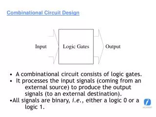
Combinational Circuits Design Procedure • 1. Specification (Requirement) • Write a specification for what the circuit should do e.g. add two 4-bit binary numbers • Specify names for the inputs and outputs • 2. Formulation • Convert the Specification into a form that can be Optimized • Usually as a truth table or a set of Boolean equations that define the required relationships between the inputs and outputs • 3. Logic Optimization • Apply logic optimization (2-level & multi-level) to minimize the logic circuit • Provide a logic diagram or a netlist for the resulting circuit using ANDs, ORs, and inverters
Combinational Circuits Design Procedure • 4. Technology Mapping and Design Optimization • Map the logic diagram or netlist to the implementation technology and gate type selected, e.g. CMOS NANDs • Perform design optimizations of gate costs, gate delays, fan-outs, power consumption, etc. • Sometimes this stage is merged with stage 3 • 5. Verification • Verify that the final design satisfies the original specification- Two methods: • Manual: Ensure that the truth table for the final technology-mapped circuit is identical to the truth table derived from specifications • By Simulation: Simulate the final technology-mapped circuit on a CAD tool and test it to verify that it gives the desired outputs at the specified inputs and meets delay specs etc.
BCD to Excess 3 Code Converter • 1. Specification • Transforms BCD code for the decimal digits (0-9) to the corresponding Excess-3 code • BCD code words for digits 0 through 9: 4-bit patterns 0000 to 1001, respectively • Excess-3 code words for digits 0 through 9: 4-bit patterns obtained by adding 3 (binary 0011) to each BCD code input • 2. Formulation • In the form of a truth table: Variables • BCD: A,B,C,D Excess-3: W,X,Y,Z • Don’t Cares: BCD 1010 to 1111
BCD to Excess 3 Code Converter • 3. Optimization • 2-level usingK-maps
BCD to Excess 3 Code Converter • 3. Logic Optimization (continued) • Start with SOPs (2-level) from the K-maps: • Extracting a common factor:
BCD to Excess 3 Code Converter • Technology Mapping • Use a library containing inverters, 2-input NAND, 2-input NOR, and 2-2 AOI gates
BCD to Excess 3 Code Converter • 5. Verification • Find the SOP Boolean equations from the final technology mapped circuit • Find the truth table from these equations • Compare it with the specification truth table • Finding the Boolean Equations
BCD to Excess 3 Code Converter • 5. Verification- Manual, Continued: The circuit truth table from the equations - Compare it with the specification truth table: The tables match!
BCD to Excess 3 Code Converter • 5. Verification- by Simulation: Procedure • Use a schematic editor or text editor to enter a gate level representation of the final circuit • Use a waveform editor or text editor to enter a test consisting of a sequence of input combinations to be applied to the circuit • This test should guarantee the correctness of the circuit if the simulated responses to it are correct • Generation of such a test can be difficult, and sometimes people apply all possible “care” input combinations
BCD to Excess 3 Code Converter • 5. Verification- by Simulation: Final Circuit Schematic
BCD to Excess 3 Code Converter • Run the simulation of the circuit for 120 ns • Do the simulation output combinations match the original specification truth table?
Iterative (Repetitive) Arithmetic Combinational Circuits • An iterative array can be in a single dimension (1D) or multiple dimensions (spatially) • Iterative array takes advantage of the regularity to make design feasible • Block Diagram of a 1D Iterative Array
4-bit Ripple-Carry Adder (RCA) • A 4-bit Ripple-Carry Adder made from four 1-bit Full Adders: • N-bit Ripple-Carry Adder:
Iterative Design Example • It is required to design a combinational circuit that computes the equation Y=3*X-1, where X is an n-bit signed 2's complement number • This circuit can be designed by assuming that we have a borrow feeding first cell or by representing -1 in 2's complement as 11…11 and adding this 1 in each cell. • We will follow the second approach. We need to represent carry-out values in the range 0 to 3. Thus, we need twosignals to represent Carry out values.
Decoders • A decoder is a circuit that decodes an input code. Given a binary code of n-bits, a decoder will tell which code is this out of the 2n possible codes. • A decoder may have enable line • In general, output i equals 1 if and only if the input binary code has a value of i. • Thus, each output line equals 1 at only one input combination but is equal to 0 at all other combinations. • Thus, the decoder generates all of the 2nminterms of n input variables
2-to-4 Decoder • A 2-to-4 decoder contains two inputs denoted by A1 and A0 and four outputs denoted by D0, D1, D2, and D3. • For each input combination, one output line is activated, that is, the output line corresponding to the input combination becomes 1, while other lines remain inactive
2-to-4 Decoder with Enable • Attach m output-enabling gates opened by the EN input • Note use of X’s to denote both 0 and 1 at the inputs • Combination containing two X’s represent four input binary combinations
Multiplexers: 2n-to-1 • A multiplexer (MUX) selects information from one of 2n input line and directs it toward a single output line. • A typical multiplexer has: • 2n information inputs (I(2n – 1), … I0) (to select from) • 1 Output Y (to select to) • n select control (address) inputs (Sn - 1, … S0) (to select with) • Implemented using decoders • MUX selection circuits can be duplicated m times (with the same selection controls in parallel) to provide m-wide data widths
2-to-1 MUX • The single selection variable S has two values: • S = 0 selects input I0 • S = 1 selects input I1 • 3-input K-map optimization gives the output equation: • The circuit: • Can be seen As: 1-to-2 decoder + Enabling + Selection
4-to-1 MUX • A 4-to-1 MUX can be implemented using three 2-to-1 MUXs. • F = s1’s0’ I0 + s1’s0 I1 + s1s0’ I2 + s1s0 I3 = s1’ (s0’ I0 + s0 I1)+ s1 (s0’ I2 + s0 I3)
Implementing Functions using Multiplexers • Using Shanon’s Expansion we can implement any function using any sizes of multiplexers • Example: f = ab + ac + bc • fa = b + c • fa’ = bc • F = a fa + a’ fa’ = a (b + c) + a’ (bc) • 2x1 MUX: f = a [ b (1) + b’ (c) ] + a’ [ b (c) + b’ (0) ] • Three 2x1 Muxs • 4x1 MUX: f = a b (1) + a b’ (c) + a’ b ( c) + a’ b’ (0)