Download
1 / 22
280 likes | 639 Vues
Radar Altimeter Fundamentals and Near-Shore Measurements. A brief commentary on well-known concepts, presented to help unify terminology and focus discussions in this Workshop. Endorsers include WHF Smith, P Callahan, P Thibaut. R. Keith Raney keith.raney@jhuapl.edu. The Playing Field.

E N D
Radar Altimeter Fundamentals and Near-Shore Measurements A brief commentary on well-known concepts, presented to help unify terminology and focus discussions in this Workshop Endorsers include WHF Smith, P Callahan, P Thibaut R. Keith Raney keith.raney@jhuapl.edu
The Playing Field • Pertinent parameters: • SSH, SWH, WS, other* • Averaging* • Resolution* • Antenna pattern (full) • Pulse-limited footprint • Radiometer pattern(s) • Propagation delays • Waveform integrity • etc • * Themes of this brief (Acknowledgement CNES/D. Ducros)
Outline • Fundamental background concepts • Replay in the coastal environment • Summarize main themes
Fundamental background concepts • Replay in the coastal environment • Summarize main themes
“Gotchas” in the near shore The Altimeter as a Radar • Fundamental radar parameters* • Range resolution(1/Bandwidth) (single pulse) ~ 50 cm • Footprint resolution: Pulse-limited (~2 km - ~10 km) • Antenna Beamwidth(-3 dB typically ~ 15 km) • Single waveform(backscatter from one transmitted pulse) • Waveform == |compressed & detected received time series|2 • Coherent self-noise (speckle) => signal/speckle ratio = 1 • Averaged waveforms (Nstatistically independent waveforms) • Coherent self-noise (standard deviation) reduced by 1/sqrt(N) • Presumes that the geophysical signal remains highly correlated among the ensemble of waveforms averaged *Altimeter-dependent
Averaged Waveform PDFs • Gamma Distribution(N statistically independent looks) • Normalized to mean = 1 • Standard deviation = sqrt(1/N) • Large N Approximation(Stirling)
Waveform PDFs (Examples) All radars are “precision-challenged” N is the number of statistically-independent samples averaged for a given measurement
Accuracy vs Precision ACCURACY and PRECISION two terms in common use (and mis-use) in radar altimetry; fundamental concepts that apply especially to near-shore measurements Standard deviation Variance (STD2) Logical synonyms Mean “Average”
Precision and Accuracy Trends Accuracy (cm) Precision (cm) 10 100 Height PRECISION(instrument dependent) is the essential measurement attribute for geodesy, bathymetry, and mesoscale oceanography Conventional altimeter lower “limit” Height ACCURACY (orbit-dependent) is the essential attribute of global topographic studies and climatology (e.g annual sea level rise) 1 10 Sun-synchronous orbit lower “limit” Delay-Doppler break-through 0.1 1 1975 1985 1995 2005 GEOS-3 GFO ERS-1 Geosat Seasat Delay-Doppler TOPEX ENVISAT ERS-2 Jason-1
Precision vs Resolution Variance x Resolution > Constant PRECISION and (Spatial) RESOLUTION Fundamental trade-off, a measurement Uncertainty Principle It follows from information theory that resolution and precision each require bandwidth (channel capacity). Hence, any system imposes an upper bound on their product Consequence 1: Application requirements need to specify BOTH measurement resolution and precision requirements Consequence 2: Radar altimeters need to specify achievable resolution and precision that can be realized simultaneously with a given measurement
Typical RA-2 (Envisat) Waveform This “hash” is dominated by speckle noise that remains after averaging (20 Hz data ~ 100 looks) Slope of the waveform tail is due to antenna pattern weighting, to mis-pointing of the antenna, and/or to sea surface specularity The tail of the waveform comes from sea surface backscatter up to 8 km - 10 km from nadir* Courtesy, CLSRamonville Saint-AgneFrance *Altimeter/altitude-dependent
ALT Measurements The familiar idealized model (Brown function) Power Backscatter power => WS Leading-edge slope => SWH Time delay to track point => SSH Accuracy objective: 1 part in 107 The challenge: convert time delay to distance, “accurately” 0 Round-trip delay time Additive noise Transmitted pulse (after compression)
Fundamental background concepts • Replay in the coastal environment • Summarize main themes
Issues: ALT Near Shore Selected examples Facts Consequences Near-shore waveform corruption Large radiometer footprint may spoil WVR estimates Antenna beamwidth* ~ 18 km Sample posting rate @ n Hz => along-track footprint length (DSWH + 6.7/n) km Shorter correlation lengths of temporal/spatial features Need adaptive or special tracker treatment, and/or re-tracking SSH accuracy compromised WS, SWH measurement reliability may suffer for near-shore observations Along-track spatial resolution* can never be better than the pulse-limited footprint diameter DSWH (> 2 km) Compromised measurement precision *Altimeter/altitude-dependent
Offshore histogram Onshore histogram Probability(fine-gate tracking) Typical results from a traditional on-board tracker Fine-gate tracking: Rule based on a set of gate values that fit expected waveform shapes; precision ~2 cm (low SWH). Alternative: threshold tracking; precision ~50 cm (one gate width) Based on a JHU/APL analysis of TOPEX performance approaching and leaving shorelines (F. Monaldo, SRO96M15 August 30, 1996)
Histogram of WVR Corruption Method: Onset of departure from trended WVR data along a 350-km segment of track Based on an analysis of 162 TOPEX passes over instrumented off-shore buoys (F. Monaldo, JHU/APL, SRO97M05, Jan 31, 1997)
) ) ) ) ) ) ) Conventional ALT footprint scan Vs/c RA pulse-limited footprint in effect is dragged along the surface pulse by pulse as the satellite passes overhead. The effective footprint dilates with longer integration time
1 Hz Less Averaging = Worse Precision Increased waveform rate implies larger measurement standard deviation Example: SWH precision of 4 cm at 1 Hz, grows to 18 cm at 20 Hz Comment: This is the lower bound. Wave profile and other factors may induce further degradation.
Fundamental background concepts • Replay in the coastal environment • Summarize main themes
Principal Themes Radar altimetry in the near-shore • Averaging • Shorter correlation length and time of oceanic features • Loss of temporal and spatial degrees of freedom means less averaging; the inherent radar self-noise grows larger • Precision • Less averaging => poorer precision • Simultaneous fine precision and fine resolution may be challenging • Accuracy • Weakening/failure of path length correction methodologies • AND Waveform Corruption • Influence from land backscatter (main lobe or side-lobes) • Oceanic surface may have anomalous profiles