Surface Wind Fields from Satellite Radar and Radiometer Measurements
720 likes | 939 Vues
Surface Wind Fields from Satellite Radar and Radiometer Measurements. Abderrahim Bentamy Laboratoire d’Océanographie Spatiale IFREMER Brest France. Acknowledgement. Denis Croizé-Fillon (IFREMER) Pierre Queffeulou (IFREMER) Marcos Portabella (UTM – CSIC) CERSAT NASA / JPL

Surface Wind Fields from Satellite Radar and Radiometer Measurements
E N D
Presentation Transcript
PORSEC 2010 Taiwan Tutorial Surface Wind Fields from Satellite Radar and Radiometer Measurements Abderrahim Bentamy Laboratoire d’Océanographie Spatiale IFREMER Brest France
PORSEC 2010 Taiwan Tutorial Acknowledgement • Denis Croizé-Fillon (IFREMER) • Pierre Queffeulou (IFREMER) • Marcos Portabella (UTM – CSIC) • CERSAT • NASA / JPL • SAF OSI / KNMI • ESA • CNES
Estimation of surface parameters from satellite data • Several Human activities and applications request high quality of surface fluxes at global and regional scales : • Climate variability • Ocean and Weather forecasting • Ship routing • Oil production • Fisheries • Food production • Extreme event detection and impact
Need of Accurate Surface Winds Wind speed and direction (orcomponents) • Wind Stress • Surface Winds • Air Humidity • Air and Surface Temperatures • Latent Heat Flux • Surface Winds • Air Humidity • Surface Humidity • Sensible Heat Flux • Surface Winds • Air Temperature • Sea Surface Temperature
Ocean Wind Vector Requirements (SoW, ESA, 2010) No Available Satellite Instrument Meets All Requirements
PORSEC 2010 Taiwan Tutorial Surface Wind Measurements ALADIN QuikSCAT Credit NOAA BLENDED Credit Météo-France
PORSEC 2010 Taiwan Tutorial Lecture Purpose • Aims • To learn about the basic methods used to estimate surface winds from scatterometers and radiometers • To appraise global ocean wind datasets from satellites • To understand how to confront in situ, numerical model, and remotely sensed flux data in the context of scientific studies and operational applications • Objective : Understanding what satellite radars and radiometers actually measure, and how the surface parameters derived from remotely sensed measurements are useful.
PORSEC 2010 Taiwan Tutorial Outline of Lecture • Methods of retrieving surface windspeeds and directions from satellite measurements • Calibration / Validation • Accuracy of surface Wind retrievals Part 1 • Enhancement of Spatial and temporal resolution • Applications Part 2
PORSEC 2010 Taiwan Tutorial Satellite Instruments • Scatterometers • Surface Wind Vector (Wind Speed and Direction) • Radiometers • Surface Wind Speed • Surface Wind Vector • Altimeters • Surface Wind Speed • SAR • Surface Wind Vector (Wind Speed and Direction)
PORSEC 2010 Taiwan Tutorial Scatterometers QuikScat (SeaWinds) ERS-1/2 ADEOS-1 (NSCAT) ADEOS-2 (SeaWinds) METOP-A (ASCAT) OceanSat-2
PORSEC 2010 Taiwan Tutorial Specifications • Polar Orbits • Sun-Synchronous • Altitude of 800km • Two observations / day • Microwave Measurements • Most ocean regions are covered with clouds 75% of time! • Microwaves “see” through clouds and atmosphere at wavelengths of 1-5cm. • Microwaves sensitive to sea surface roughness
Scatterometer measurement : Examples • NSCAT • Polarization : V; H • Swath : 2x600km • WVC Resolution : 50 km (25km) • Coverage : 78% • Period : 1996 – 1997 • ERS-1/2 • Polarization : VV • Swath : 500km • WVC Resolution : 50 km • Coverage : 41% • Period : 1991 - 2001 • QuikSCAT • Polarization : V; H • Swath : 1800km • WVC Resolution : 25 km (12.5km) • Coverage : 92% • Period : 1999 - 2009 • ASCAT • Polarization : V • Swath : 550 km • WVC Resolution : 50km / 25 km • Coverage : 84% • Period : 2006 - Present
PORSEC 2010 Taiwan Tutorial Scatterometer Principle • Wind creates small waves on the ocean surface (capillary waves) which in the absence of wind will continue to propagate. • If wind continues, waves will grow in size and increase in wavelength and height to become ultra-gravity waves and eventually gravity waves. • A water surface affected by wind will have a spectrum of surface waves, e.g, multiple wavelengths and heights • Microwave EM energy has been shown through wave tank experiment to constructively interfere or resonate with surface capillary and ultra-gravity waves. • This phenomenon is known as Bragg Scattering
Scatterometer measurements • Scatterometers are active microwave sensors: they send out a signal and measure how much of that signal returns after interacting with the target. Microwaves are Bragg scattered by short water waves; the fraction of energy returned to the satellite (backscatter) is a function of wind speed and wind direction. • The main scatterometer measurements are the backscatter coefficients calculated as a ratio between the emitted power Pe and the received one Pr : : the wavelength, G the antenna gain, A the radar footprint, R the distance between the sensor and the reached target.
PORSEC 2010 Taiwan Tutorial Backscatter coefficient Behaviors ° as a function of Wind Speed and Incidence Angle • 0 increases with wind speed. The increasing gradient is higher for surface winds less than 12m/s than for higher wind conditions.
PORSEC 2010 Taiwan Tutorial Backscatter coefficient Behaviors ° as a function of Wind Direction and Speed • Due to electromagnetic interactions 0 are different whether the measurement is made upwind (=0°), downwind (= 180°), and crosswind (=90° or 270°)
PORSEC 2010 Taiwan Tutorial Scatterometer Geophysical Relationships GMF : • : Wind direction wrt azimuth • : Incidence angle • U : Wind Speed • P: Polarization • Fc : Frequency GMF Determination Calibration / Validation
PORSEC 2010 Taiwan Tutorial Calibration and Validation Issues:Collocation Procedures • Buoy Networks • NDBC (NOAA) • MFUK (MFUK) • TAO (PMEL/NOAA) • PIRATA (INPE/IRD/PMEL) • RAMA (PMEL) • In-Situ • COADS • Experiments (Fastex; KNORR; EPIC; PACS N/S; FETCH; POMME; EQUALANTE;EGEE(AMA)) • Multi-Satellite
PORSEC 2010 Taiwan Tutorial Moored Buoys
PORSEC 2010 Taiwan Tutorial Collocation Procedure • The collocation consists in grouping measurements close in space and time from various sensors (or other data sources like numerical model outputs). Two measurements are said to be close if they are below a given distance and time difference. These collocation criteria are set according to each sensor geometry as well as each satellite orbital parameters; For each collocated measurement, a selection of parameters from each source data product (associated to a sensor) is provided.
PORSEC 2010 Taiwan Tutorial Scatterometer Geophysical Relationships GMF : Buoy Wind Speed Range 8m/s
PORSEC 2010 Taiwan Tutorial Scatterometer Geophysical Relationships GMF : Buoy Wind Speed Range 3m/s
PORSEC 2010 Taiwan Tutorial Scatterometer Geophysical Relationships GMF : Buoy Wind Speed Range 12m/s
PORSEC 2010 Taiwan Tutorial Scatterometer Geophysical Relationships(Bentamy et al, 2008) 0u = A0 + A1 + A2; 0d = A0-A1+A2; 0c = A0-A2 Behaviours of fore-beam (top), mid-beam (middle), and aft-beam (bottom) A0, A1, and A2 as a function of incidence angle for three wind speed ranges (3m/s (blue), 8m/s (red), and 12 m/s (black)). A0 = ( u + d + 2c)/4 A1 = ( u - d)/2 A2 = ( u + d - 2c)/4
PORSEC 2010 Taiwan Tutorial Scatterometer Surface Wind Vector Retrievals (1) Assumptions • 0 = 0P + 0P states for « truth » backscatter coefficient. is the error measurement is assumed Gaussian with zero mean and variance . • 0P is related to GMF through : 0P = 0mod + mod 0mod is backscatter coefficient value estimated from GMF mod is the model error assumed Gaussian with mod variance. For given wind speed and direction over WVC, the difference between measured and simulated backscatter coefficients is calculated: =0 - 0mod Assuming that instrumental and model errors are independent, is Gaussian with zero mean and variance = + mod
PORSEC 2010 Taiwan Tutorial Scatterometer Surface Wind Vector Retrievals (2) Therefore the probability density function of constrained by 0 : P(/0 ) = P(/{U,}) = (8) Let is consider N the number of 0 over WVC (3 in ERS case), and the corresponding are independent. The conditional probability is provided by: P(1 … N /{U,}) = (9) The maximum likelihood estimator (MLE) criterion implies that the solution {U,} is the local minimum of P. In general, over each WVC the wind speed and direction solutions are determined as a maximum of the following function : J(U,) = (10) J is related to P through logarithm transform. The algorithm proposes up 4 solutions, called ambiguities. The most probable vector is indicated as theselected wind vector for the specific WVC. This selection is mainly based on the MLE and quality control (QC)
PORSEC 2010 Taiwan Tutorial Scatterometer Surface Wind Vector Retrievals (3) Up 4 Solutions
PORSEC 2010 Taiwan Tutorial Scatterometer Surface Wind Vector Retrievals : Ambiguity issue • If scatterometer observes a particular cross section 0() at an azimuthal angle relative to the wind, all points on the curve are possible wind vectors that yield the observed cross section. If the oceanic area is observed from three different directions, -45°, , +45° (ERS case) as shown in the example, 2 or 4 possible wind vectors satisfy the observations, because scatter is only weakly anisotropic Wind 8m/s SA T 120°
PORSEC 2010 Taiwan Tutorial QuikSCAT Swath Wind Data
Examples of the Scatterometer Retrieved Surface Wind Vectors. The Abdu Salam Internal Center for Theoretical Physics. Trieste Italy. February 2009
PORSEC 2010 Taiwan Tutorial Accuracy issue : Statistical parameters • Statistical moments : • Linear moments : • Regression parameters : • Wind direction : • Test Hypothesis : Mean, variance, correlation coefficient, and distribution
PORSEC 2010 Taiwan Tutorial Scatterometer Wind Accuracy • Comparison of the wind speeds (left panel) and directions (right panel)observed by ERS-1 (top), ERS-2 (middle), and QuikScat (bottom) scatterometers with 10-m buoy winds moored in the Atlantic ocean (first column), the Pacific ocean (second column), and in the Tropical oceans (third column). Tropical
PORSEC 2010 Taiwan Tutorial Special Sensor Microwave / IMAGER (SSM/I) Principle
PORSEC 2010 Taiwan Tutorial SSM/I Measurements • Main SSM/I measurement : • Definition : Brightness Temperature is a measure of the intensity of radiation thermally emitted by an object, given in units of temperature because there is a correlation between the intensity of the radiation emitted and physical temperature of the radiating body which is given by the Stefan-Boltzmann law. TA = etTs + (1-t)T’ +(1-t)(1-e)tT’ + (1-e)t²(Text - Tsol) (Stewart, 1985) Ts = Surface temperature e, (1-e) : emissivity and reflectivity T : transmissivity T’ : the vertical average of the tropospheric temperature profile From Seelye Martin, (2004)
PORSEC 2010 Taiwan Tutorial SSM/I Surface and Atmospheric Parameter Retrievals (1) • Atmospheric water vapor content • Atmospheric water liquid content (cloud) • Wind speed on ocean surfaces • Ground humidity • Rain rates • Snow surfaces detection and water content analysis • Sea-ice detection and concentration sea-ice characterization
PORSEC 2010 Taiwan Tutorial SSM/I Surface Wind Speed Retrievals (2) Schlussel, 1997 • Statistical models are used to estimate the geophysical parameters from Brightness temperatures • Wind Speed : U = 1.0969TB19V – 0.4555TB22V – 1.76TB37V + 0.786TB37H + 147.9 (Goodberlet et al, 1989) U = f(TB) + f(WV) (Bentamy et al, 1999)
PORSEC 2010 Taiwan Tutorial Examples of SSM/I Surface Wind Observations1St January 2004 3am – 9am SSM/I F13 SSM/I F14 SSM/I F15 QuikSCAT
PORSEC 2010 Taiwan Tutorial Validation of SSM/I Wind Retrievals Ussmi = f(TB, WVC) Uers = f(0)
PORSEC 2010 Taiwan Tutorial Part 1 : Summary • The remotely sensed winds provide valuable and unique source of the main surface parameter at global and regional scales • They compare well with in situ data in various geographical areas • Some improvements are needed : • Wind conditions • Rain detection • Sea State • Parameterization • Coastal • Resolutions • …
PORSEC 2010 Taiwan Tutorial Part 2 • Remotely Sensed Use : • Regional and global ocean model forcing; Process analysis; Meteorology; Operational costal and global oceanography, … • Calculation of Surface Wind Analysis Using Satellite Observations • Estimation of Surface Parameters at Regular Space/Time Resolution • Enhancement of Spatial and Temporal Resolutions
Higher Level Wind Processing • Level 3: spatio-temporally consistent wind product from a single wind source • Level 4: spatio-temporally consistent wind product from combined wind sources
PORSEC 2010 Taiwan Tutorial L3 ProductDaily Wind Fields 27th – 29th August 2005 OBSERVATIONS ANALYSIS
2nd EPS/METOP 20 - 22 May 2009 Barcelona Spain Daily Gridded Wind Field Estimation Scheme SCAT data • only valid (0, U, u, v) • wind selection • sampling Data selection • stress Additional data computation t Neighbours search Xi y x X0 (x0, y0, t0) Gridding Objective analysis Masks (land, ice…) Variogram Winter Summer Geographic grids
2nd EPS/METOP 20 - 22 May 2009 Barcelona Spain Gridded Wind Field Estimation Geographic grids • wind divergence • stress curl Derived quantities computation Quality control Geographic grids Quality Assessment Validation graphs
PORSEC 2010 Taiwan Tutorial Accuracy Issue : Difference Sources • Raw data • Calibration / Validation Procedures • Spatial and Temporal Resolutions • Estimation of basic variables : Winds, Humidity, Sea Surface and Air Temperatures • Analysis Methods • Flux Algorithms • … In-situ / satellite Differences
PORSEC 2010 Taiwan Tutorial Error related to the Objective Method Satellite Sampling Scheme • Use of simulated satellite data from buoy measurements or from ECMWF analysis • Temporal Sampling Impact : • <X> : Time - Averaged surface parameter from Hourly Buoy Data • <X’> : Time - Averaged surface parameter from Hourly Buoy Data close to satellite passes • Rms of <X> - <X’>