Download
1 / 22
250 likes | 443 Vues
ACCURACY OF COMPOSITE WIND FIELDS DERIVED FROM A BISTATIC MULTIPLE-DOPPLER RADAR NETWORK Shinsuke Satoh and Joshua Wurman School of Meteorology, University of Oklahoma. 1. INTRODUCTION. What is a bistatic Doppler network? A Doppler network to measure 3D wind field, that

E N D
ACCURACY OF COMPOSITE WIND FIELDS DERIVED FROM A BISTATIC MULTIPLE-DOPPLER RADAR NETWORK Shinsuke Satoh and Joshua Wurman School of Meteorology, University of Oklahoma
1. INTRODUCTION What is a bistatic Doppler network? A Doppler network to measure 3D wind field, that consists of one transmitting Doppler radar and one or more passive low-gain, non-scanning receivers. Objectives (1) To investigate the influence of several factors on accuracy of composite wind fields (2) To eliminate multiple and sidelobe scattering, a bistatic antenna pattern is estimated using time-averaging reflectivity (3) To propose a practical composite method for bistatic multiple-Doppler radar network
Advantages and limitations [+] Easy and inexpensive installation [+] All Doppler velocities measured from Individual volumes simultaneously ( We do not need to assume steady state. ) [+] Use only one frequency [-] Less sensitive to weak echoes ( Usually, this is not serious problem because a Doppler signal can be obtained from a minimum detective intensity. ) [-] More sensitive to multiple scattering and sidelobe contamination
Data for analysis observed in Kansas during CASES-97 05/19/97, 0700-1030GMT convective and stratiform echo, SPOL and one bistatic site (NO) 05/30/97, 0200-0600GMT stratiform echo, SPOL and three bistatic sites (NO, CE, SO) EL angles: 0.5, 1.0, 1.4, 2.4, 3.4 deg Locations of main radar (NCAR SPOL) and three bistatic receiver sites (NO, CE, SO). Line between SPOL and each bistatic site indicate a baseline. Circles show dual-Doppler analysis areas by scatter angles (b /2) of 25 deg.
t + t V D R S t R2 R1 b/2 b/2 R T BL 2. BISTATIC GEOMETRY Schematic diagram of transmitter(T)-scatterer(S)-receiver(R) geometry and Doppler velocity vector (VDR) measured by a bistatic receiver. Where, b is the angle between T-S and R-S, Dashed lines indicate constant delay time surfaces form ellipsoids with foci at T and R. Since the VDR is proportional to the difference in pathlength between two successive pulses which time interval is t, the VDR is oriented perpendicular to the ellipsoids. The direction of VDR is represented by grad (t) vector, and its angle is b /2.
PPI (EL=0.5 deg) displays of (a) Distance of T-S-R (R1+R2) or constant delay time the light speed, (b) Azimuth from a bistatic site, (c) Azimuth of bistatic Doppler velocity, (d) Scatter angle ( /2), where cos( )=(R12 + R22 - BL2) / 2 R1 R2, (e) Expansion factor of Doppler velocity: (cos( /2))-1 , (f) Expansion factor of volume length: (cos2( /2))-1 .
PPI (EL=0.5 deg) displays of (g) Elevation from a bistatic site, (h) Elevation of bistatic Doppler velocity, (i) Scatter angle against incident E-Vector of V-polarization: I = I0 sin2 , (j),(k),(l) are same as (g),(h),(I) ,respectively, except EL=3.4 deg.
(1) Eliminate noise data using normarized coherent power (NCP) (2) Eliminate multiple and sidelobe scattering data using an estimated antenna pattern (3) Unfolding Doppler velocity (Multiply expansion factor by the velocity afterward) (4-1) Dual-Doppler processing on radar coordinates (4-2) Coordinates conversion from R-into X-Y-Z (4’-1) Coordinates conversion from R- into X-Y-Z (4’-2) Dual-Doppler processing on Cartesian coordinates 3. PROCEDURE OF WIND VECTOR CALCULATIONS
Variational Method in over-determined cases Continuity equation as a strong constraint Observed winds from dual-Doppler pairs as weak constraints When observed Doppler velocities (un,vn) include few vertical components,
4. Eliminate multiple and sidelobe scattering Strong echo may cause multiple and sidelobe scattering. These abnormal scattering will disappear due to time-integration of bistatic Ze. The distribution of enough time-average Ze indicates the bistatic antenna pattern. Multiple scattering echo Sidelobe echoes Mainlobe Sidelobe Subtract averaged BIST-Ze from averaged SPOL-Ze Estimated Bist Ant. Pattern If (BIST-Ze + Ant-Pattern) is larger than observed SPOL-Ze, the BIST-data may be abnormal scattering.
(a)(b)(c) Time series of vector winds superimposed on SPOL-Ze on EL-0.5 deg. , (d)(e)(f) magnitude of wind speed. Elimination processes of multiple and sidelobe scattering have not been done.
(a)(b)(c) Time series of vector winds superimposed on BIST-Ze on EL-0.5 deg. , (d)(e)(f) magnitude of wind speed, as a result of eliminating multiple and sidelobe scattering.
Comparison among three wind fields from (a)SPOL-NORTH, (b)SPOL-CENTER, (c)SPOL-SOUTH. Contours represent scatter angle ( /2) of 20, 30, 40, and 50 deg. Magnitude of the vector difference (d) between SPOL-NORTH and SPOL-CENTER, (e) between SPOL-NORTH and SPOL-SOUTH, (f) between SPOL-CENTER and SPOL-SOUTH.
(g) between SPOL-NORTH and COMPOSITE, (h) between SPOL-CENTER and COMPOSITE, (i) between SPOL-SOUTH and COMPOSITE. (j),(k),(l) are NCPs of NORTH, CENTER, SOUTH, respectively.
Scatter diagram of magnitude vector difference against the smaller scatter angle (/2).
SUMMARY (1) A bistatic antenna pattern estimated by time- averaging is useful in eliminating multiple and sidelobe scattering. (2) Since the scatter angle ( /2) dominates accuracy of wind vector synthesis, it is used for making composite as a weight function within an over-determine region. Future works - The Influence of the expansion factor near a base-line (large /2) - Problems of high elevation angle: antenna pattern and an angle with incident E-vector