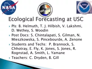
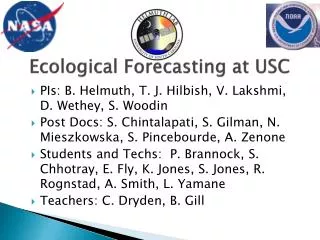
Ecological Forecasting at USC
Ecological Forecasting at USC. PIs: B. Helmuth, T. J. Hilbish, V. Lakshmi, D. Wethey, S. Woodin Post Docs: S. Chintalapati, S. Gilman, N. Mieszkowska, S. Pincebourde, A. Zenone Students and Techs: P. Brannock, S. Chhotray, E. Fly, K. Jones, S. Jones, R. Rognstad, A. Smith, L. Yamane

Ecological Forecasting at USC
E N D
Presentation Transcript
Ecological Forecasting at USC • PIs: B. Helmuth, T. J. Hilbish, V. Lakshmi, D. Wethey, S. Woodin • Post Docs: S. Chintalapati, S. Gilman, N. Mieszkowska, S. Pincebourde, A. Zenone • Students and Techs: P. Brannock, S. Chhotray, E. Fly, K. Jones, S. Jones, R. Rognstad, A. Smith, L. Yamane • Teachers: C. Dryden, B. Gill
Ecological and Environmental Gradients Variable of interest (e.g. Temperature) Space (e.g. Latitude) Time (years, decades, centuries)
Reality Variable of interest (e.g. Temperature) Space (e.g. Latitude) Time (years, decades, centuries)
Variable of interest (e.g. Temperature) Space (e.g. Latitude) Time (years, decades, centuries)
Analyzing Environmental Signals • Environmental “gradients” exist comprise signals of different frequencies; however, we often only pay attention to the low frequency components (e.g. long term trends) • E.g. Effects of PDO, ENSO in time counteract or amplify warming trends; effects of factors such as upwelling, local fog, etc. in space can trump latitude • Do we really know how patterns of environmental stressors change in space and time? • What is signal and what is noise? (and what frequencies do we need to measure and record?)
To an organism, all weather, climate, and climate change is local, at the level of the microhabitat Seastar at ~12°C Mussel at ~21°C
“Signal” is determined by the behavior, morphology, and physiology of the organism • Two organisms exposed to identical microclimates can often show very different body temperatures • Physiological effects are both direct and indirect: • Mussels die at body temperatures in excess of 36°C when exposed at low tide (KA Smith) and/or when food supply is low (Schneider et al.) and/or when winter water temps <10.5°C (Wethey) • Seastars reduce foraging on mussels when exposed to aerial body temperatures above 14°C (Pincebourde et al.)
Experimental Physiological and Ecological Data Climate Models and Weather Data Theoretical Models of Organism Body Temperature Fundamental Niches Primary Space Occupiers Invasive spp. Keystone spp. Species Interactions (Competition, Predation, Facilitation) Realized Niches (spatially and temporally explicit maps of distribution, abundance, and growth) Make and Test Hypotheses in space and Time
What is sufficient resolution so that we are not ignoring important “signal”?
Mussel temperatures have been steadily increasing since 2000: why?
Patterns in Environmental Variables often different from those relevant to the organism • Not surprisingly, magnitude of variables such as air and water temperature often vary from physiologically relevant factors such as body temperature • However, patterns both quantitatively and qualitatively vary
Body temperature vs air and water temperature of intertidal mussels In phase Out of phase Helmuth 2009 J. Exp. Biol.
0/year 0 to 2/year > 2/year West Coast Mussel Mortality Risk: Frequency of 36° C temperatures for at least 2 hours over 3 consecutive days Allison Smith
M gallo Moving north in English Channel Abundant in Brittany Rarer on French Biscay Coast Abundant in Iberia Cold days in winter inhibitory European Mussel Hybrid ZoneDays in January below 10.5°C from Reynolds GHRSST 0.25° 1985 2007 RW Reynolds, NOAA NCDC, GHRSST OISST-AVHRR Daily 1985-present
Present Day Barrier Dispersal Dead Dead Alive Temperature (°C) Alive Latitude
Barrier Barrier Dispersal Dead Temperature (°C) Alive Latitude
Barrier: sp 1 only Barrier: both spp. No barriers Temperature (°C) Sp. 2 threshold Sp. 1 threshold Species 2 Species 1 Latitude
Marine Protected Areas: must work now and in the future Now Climate Change Now 20-50 years Climate Change Latitude Latitude Abundance Abundance
20-50 years Now Climate Change 4) Plan network of “stepping stones” in advance By forecasting changes in abundance of key species, we can design MPAs so that distance between current and future stepping stones is set by dispersal ability of key species
Summary • Mechanistic forecasting has similar goals to statistical modeling, but does not assume all edges are set by same environmental factors • Time intensive, so focus on key “foundation” species that directly or indirectly drive patterns of biodiversity and ecosystem function • Can complement statistical approaches by targeting specific needs of resource managers
Funding • NASA grants NNG04GE43G and NNX07AF20G • NOAA Ecofore grant NA04 NOS4780264