Download
1 / 37
410 likes | 708 Vues
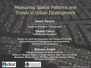
Measuring Spatial Patterns and Trends in Urban Development. Jason Parent jason.parent@uconn.edu Academic Assistant – GIS Analyst Daniel Civco Professor of Geomatics Center for Land Use Education And Research (CLEAR) Natural Resources Management and Engineering University of Connecticut

E N D
Measuring Spatial Patterns and Trends in Urban Development Jason Parent jason.parent@uconn.edu Academic Assistant – GIS Analyst Daniel Civco Professor of Geomatics Center for Land Use Education And Research (CLEAR) Natural Resources Management and Engineering University of Connecticut Shlomo Angel Adjunct Professor of Urban Planning Robert F. Wagner School of Public Service, New York University Woodrow Wilson School of Public and International Affairs, Princeton University Image courtesy of the Union of Concerned Scientists: www.ucsusa.org
The Consequences of Development Pattern and Density • Development consumes and degrades nearby natural resources. • The pattern of development influences the impact on natural resources… • “Sprawling” patterns consumes more land than traditional urban development and causes greater fragmentation of open lands. • Population density determines how much land is consumed for a given population. • Low population densities result in more land being converted to urban land cover.
Indicators of ‘sprawling’ development? • Declining spatial density of developed land • Declining population density • Increasing amount of degraded* land relative to the developed area • Increasing interspersion of developed and undeveloped land • Declining compactness of the urban area • Increasing numbers of unviable patches isolated by urbanized land * We consider land “degraded” if within 100 meters of developed land
Objectives • Develop metrics that can be used to quantify major indicators of urban sprawl. • Metrics comparable over time and for different cities • Apply metrics to a global sample of 120 cities for two time periods: circa 1990 and 2000. • Correlate metrics with socio-economic factors including income levels, political region, and city population.
Land Cover Maps • Basis for all analysis. • Derived from Landsat satellite imagery • pixel size 30 meters Color Infrared (4,5,3)
Land Cover Maps • Classified urban (developed) and water for each city for the two time periods. • “Other” is considered open (undeveloped) land.
Population data • Population data associated with administrative districts for each city. • Census data interpolated to estimate population for land cover dates.
Slope data • Slope derived from Shuttle Radar Topography Mission data. • pixel resolution of 85 meters • resampled to match land cover resolution
Spatial density of developed land • Developed land cover approximates impervious surface area. • Developed pixels classified based on percentage of land within 560 meters that is developed. • A roving neighborhood centers on each developed pixel and % developed land is calculated.
960 dev. pix = 80% 1200 total pix 560 m Urban 50-100% Developed pixels are dark gray
240 dev. pix = 20% 1200 total pix 560 m Suburban 10 – 50% Developed pixels are dark gray
40 dev. pix = 3% 1200 total pix 560 m Rural 0 – 10% Developed pixels are dark gray
Percent imperviousness vs. development density urban suburban Kauffman, G. and T. Brant. The Role of Impervious Cover as a Watershed-based Zoning Tool to Protect water Quality in the Christina River Basin of Delaware, Pennsylvania, and Maryland. University of Delaware, Institute for Public Administration, Water Resources Agency. Watershed Management 2000 Conference
Open land degraded by proximity to developed land • Close proximity of open land to developed land reduces natural resource value: • Lower quality as habitat. • Increased susceptibility to invasive species. • Less suitable as a timber resource (if forested). • Over what distances do “edge-effects” occur? • Depends on issue of interest • For habitat, ranges from 25 meters to several hundred meters depending on species. • We assume a 100 meter edge-width for general purposes in this study. • Lands within 100 meters of developed land are classified as edge open land.
Open land degraded by isolation from other non-degraded open lands • Open land may be degraded if cut-off from other open lands. • Many species require mixing between different populations. • Isolated patches may be too small to sustain viable populations for certain species. • We consider the following to be impassable to wildlife: • urban • suburban • edge open land
We assume that patches are viable if larger than 200 ha. Patches smaller than 200 ha are classified as isolated open patches. Patch size vs. habitat quality http://sof.eomf.on.ca/Biological_Diversity/Ecosystem/Fragmentation/Indicators/Size/i_wooded_patch_size_by_watershed_e.htm
Baku, Azerbaijan * Areas represented as percent of the total developed area
Population density • Measured for the developed area • Population from city administrative districts Population density (persons / ha) of developed area for Baku
Interspersion of developed and open land • Greater dispersion of developed land within open land increases the amount of open land influenced per unit of developed land. • Sprawling development patterns are expected to have greater percentage of developed land that is adjacent to open land.
Edge Index: The fraction of developed pixels that are cardinally adjacent to at least one undeveloped pixel. In other words, the fraction of pixels that make up the edge of the developed area. Interspersion of developed and open land – the Edge Index Roving window centers on each developed pixel Built-up pixels in gray Open pixels in white
960 open pix = 0.8 1200 total pix Interspersion of developed and open land – the Openness Index The Openness Index: • The average openness of developed pixels. • Openness = the fraction of land within a 560 meter radius that is undeveloped. • Roving neighborhood centers on each developed pixel.
The shape of the urban footprint • The urban footprint is the land directly impacted by the presence of development. • Irregular and non-compact footprints will create more edge and isolated open land and encourage low density development.
Compactness indices • We use several metrics for measuring compactness of a shape: • Values are normalized and range between 0 and 1 • Normalized using a circle with area equal to the shape area – the equal area circle • Most are highly correlated with each other and with people’s perception of compactness
Metrics vs. intuition Correlation Matrix 2 5 8 • Metrics are highly correlated with each other as well as with people’s intuition. • Metrics are good proxies for each other – some are easier to calculate. 7 1 3 4 9 6
The Proximity Index: Based on average distance, of all points in the urban footprint, to the center of the footprint. Normalized by the average distance (d) to center of the equal area circle with radius (r) – a circle with an area equal to that of the urban footprint. d = (2 / 3) * r Measuring Compactness: The Proximity Index Urban footprint in gray, center is black
The Cohesion Index: Based on the average distance between all possible pairs of points in the urban footprint Normalized by average distance (d) between all pairs of points within the equal area circle with radius (r). d = 0.9054 * r Measuring Compactness: The Cohesion Index Urban footprint pixels in gray, sample points in black
Measuring Compactness: The Exchange and Net Exchange Indices The Exchange Index • The fraction of the shape area that is within an equal area circle centered at the shape center. The Net Exchange Index • The fraction of the shape area that is within the netequal area circle centered at the shape center. • The net equal area circle has a buildable area (excluding water and excessive slope) equal to the urbanized area Compactness = 0.75
Urban footprints ofMinneapolis and Bangkok Minneapolis (1992) Bangkok (1994)
Increasing compactness Exchange Index for Bangkok (1994-2002) and Minneapolis (1992-2001)
Preliminary results • Sprawl tends to be inversely correlated with income level: • Developed countries have much lower population densities than developing countries. • Population density in all regions tends to decline over time. • Spatial densities seem to increase over time as the result of infill of the urban footprint. • Possibly a cyclic phenomena
Conclusions • Analysis of a global sample of 120 cities will be completed in the near future… • Will determine significance of factors believed to drive urban sprawl. • Will illuminate how urban development patterns and population densities change over time. • Metrics have potential applications in other landscape level analyses… • i.e. measuring patch compactness, interspersion of land covers, etc.
Publications • Future publications and project information will be available through the Center for Land Use Education and Research – http://clear.uconn.edu • Angel, S, J. R. Parent, and D. L. Civco. May 2007. Urban Sprawl Metrics: An Analysis of Global Urban Expansion Using GIS. ASPRS May 2007 Annual Conference. Tampa, FL • Angel, S, S. C. Sheppard, D. L. Civco, R. Buckley, A. Chabaeva, L. Gitlin, A. Kraley, J. Parent, M. Perlin. 2005. The Dynamics of Global Urban Expansion. Transport and Urban Development Department. The World Bank. Washington D.C., September.
QUESTIONS? Urban Growth Analysis:Calculating Metrics to Quantify Urban Sprawl Jason Parent jason.parent@uconn.edu Academic Assistant – GIS Analyst Daniel Civco Professor of Geomatics Center for Land Use Education And Research (CLEAR) Natural Resources Management and Engineering University of Connecticut Shlomo Angel Adjunct Professor of Urban Planning Robert F. Wagner School of Public Service, New York University Woodrow Wilson School of Public and International Affairs, Princeton University Image courtesy of the Union of Concerned Scientists: www.ucsusa.org