Download
1 / 64
640 likes | 1.04k Vues
Chapter 16 Output and the Exchange Rate in the Short Run. Supplementary Notes. Introduction. This chapter builds on the short run and long models of exchange rates to explain how output and the exchange rate are determined in the short run.

E N D
Chapter 16Output and the Exchange Rate in the Short Run Supplementary Notes
Introduction • This chapter builds on the short run and long models of exchange rates to explain how output and the exchange rate are determined in the short run. • Develop the AA-DD model (similar to the IS-LM model with a different focus)
Aggregate Demand Aggregate demand is the aggregate amount of goods and services that people are willing to buy: • consumption expenditure (C) • investment expenditure (I) • government purchases (G) • net expenditure by foreigners: the current account (CA)
Aggregate Demand (cont.) Determinants of consumption expenditure include: • Disposable income (Y-T): income from production (Y) minus taxes (T). • The marginal propensity to consume (MPC) out of disposable income is positive but less than one. • Other important determinants of consumption • Real interest rates • Wealth • They are ignored for simplicity.
Aggregate Demand (cont.) Determinants of the current account include: • Disposable income: more disposable income means more expenditure on foreign products (imports)and a reduction in CA. • Real exchange rate (EP*/P): the prices of foreign products relative to the prices of domestic products, both measured in domestic currency:
The Real Exchange Rate and the Current Account The current account measures the value of exports less the value of imports: CA ≈ EX – IM. Current account in domestic currency = PQx – EP*Qm Current account in real terms = Qx – (EP*/P)Qm EX Qx, IM (EP*/P)Qm When the real exchange rate EP*/P rises, the prices of foreign products rise relative to the prices of domestic products. • The volume of exports (Qx) rises. • The volume of imports (Qm) falls. • The value of imports in terms of domestic products (EP*/P) rises.
The Real Exchange Rate and the Current Account (cont.) • If the volumes of imports and exports do not change much, the value effect may dominate the volume effect when the real exchange rate changes. • Evidence indicates that for most countries the volume effect dominates the value effect in 1 year or longer. • Therefore, we assume that a real depreciation leads to an increase in the current account: the volume effect dominates the value effect.
Determinants of Aggregate Demand • Determinants of the current account include: • Real exchange rate: an increase in the real exchange rate increases the current account. • Disposable income: an increase in the disposable income decreases the current account.
Determinants of Aggregate Demand (cont.) • For simplicity, we assume that exogenous political factors determine government purchases G and the level of taxes T. • For simplicity, we also assume that investment expenditure I is determined exogenously. • A more complicated model shows that investment depends on the cost of borrowing for investment, the interest rate.
Current account as a function of the real exchange rate and disposable income. Consumption as a function of disposable income Investment and government purchases, both exogenous Determinants of Aggregate Demand (cont.) • Aggregate demand is therefore expressed as: D = C(Y – T) + I + G + CA(EP*/P, Y – T) • Or more simply: D = D(EP*/P, Y – T, I, G)
Determinants of Aggregate Demand (cont.) Determinants of aggregate demand include: • Real exchange rate: an increase in the real exchange rate increases the current account, and therefore increases aggregate demand for domestic products. • Disposable income: an increase in the disposable income increases consumption, but decreases the current account. • Since total consumption expenditure is usually greater than expenditure on foreign products, the first effect dominates the second effect. • As income increases for a given level of taxes, aggregate consumption and aggregate demand increases by less than income. • E.g., MPC = 0.8, MPM = 0.2. Then, Y by$100 C by $80 and CA by $20 AD by $60
Aggregate demand as a function of the real exchange rate, disposable income, investment, government purchases Value of output, income from production Equilibrium condition Short Run Equilibrium for Aggregate Demand and Output • Equilibrium is achieved when the value of output Y (and income from production) equals aggregate demand D. Y = D(EP*/P, Y – T, I, G)
Output is greater than aggregate demand: firms decrease output Aggregate demand is greater than production: firms increase output Short Run Equilibrium for Aggregate Demand and Output (cont.)
Short Run Equilibrium and the Exchange Rate: DD Schedule • How does the exchange rate affect the short run equilibrium of aggregate demand and output? • With fixed domestic and foreign price levels, a rise in the nominal exchange rate makes foreign goods and services more expensive relative to domestic goods and services. • A rise in the exchange rate (a domestic currency depreciation) increases the aggregate demand for domestic products. • In equilibrium, aggregate demand matches output.
Short Run Equilibrium and the Exchange Rate: DD Schedule (cont.)
Short Run Equilibrium and the Exchange Rate: DD Schedule (cont.)
Short Run Equilibrium and the Exchange Rate: DD Schedule (cont.) DD schedule • shows combinations of output and the exchange rate at which the output market is in short run equilibrium (aggregate demand = aggregate output). • slopes upward because a rise in the exchange rate causes aggregate demand and aggregate output to rise.
Shifting the DD Curve Changes in the exchange rate cause movements along a DD curve. Other changes cause it to shift: • Changes in G: more government purchases cause higher aggregate demand and output in equilibrium. Output increases for every exchange rate: the DD curve shifts right.
Shifting the DD Curve (cont.) • Changes in T: higher taxes generally decrease consumption expenditure, decreasing aggregate demand and output for every exchange rate: the DD curve shifts ____. • Changes in I: higher investment demand shifts the DD curve ____. • Changes in P relative to P*: higher domestic prices relative to foreign prices shift the DD curve ____.
Shifting the DD Curve (cont.) • Changes in C: willingness to consume more and save less shifts the DD curve ____. • Changes in demand for domestic goods relative to foreign goods: willingness to consume more domestic goods relative to foreign goods shifts the DD curve ____.
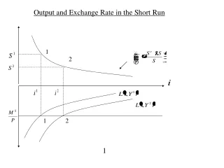
Short Run Equilibrium for Assets We consider two asset markets when considering asset market equilibrium: • Foreign exchange market • interest parity determines equilibrium: R = R* + (Ee – E)/E • Money market • real money supply and demand determine equilibrium: Ms/P = L(R, Y) • A rise in income and output causes real money demand to increase.
Short Run Equilibrium for Assets: AA Curve • When income and output increase, • money demand increases, • leading to an increase in the domestic interest rate, • leading to an appreciation of the domestic currency. • An appreciation of the domestic currency is a fall in E. • When income and output decrease, the domestic currency depreciates and E rises. • The inverse relationship between output and exchange rates needed to keep the foreign exchange market and money market in equilibrium is summarized as the AA curve.
Equilibrium exchange rate in foreign exchange market; Equilibrium output in money market. Short Run Equilibrium for Assets: AA Curve (cont.)
Shifting the AA Curve • Changes in Ms: an increase in the money supply reduces interest rates, causing the domestic currency to depreciate (a rise in E) for every Y: the AA curve shifts up (right).
Exchange rate, E 1 2 AA AA’ Y1 Output, Y Y2 Shifting the AA Curve (cont.)
Shifting the AA Curve (cont.) • Changes in real money demand: if domestic residents are willing to hold greater real money balances, interest rates rise, leading to an appreciation of the domestic currency (a fall in E): the AA curve shifts _____. • Changes in R*: An increase in the foreign interest rates makes foreign currency deposits more attractive, leading to a depreciation of the domestic currency (a rise in E): the AA curve shifts _____.
Shifting the AA Curve (cont.) • Changes in Ee: if market participants expect the domestic currency to depreciate in the future, foreign currency deposits become more attractive, causing the domestic currency to depreciate (a rise in E): the AA curve shifts _____. • Changes in P: An increase in the domestic price level decreases the real money supply, increasing interest rates, causing the domestic currency to appreciate (a fall in E): the AA curve shifts _____.
Putting the Pieces Together: the DD and AA Curves A short run equilibrium means the nominal exchange rate and level of output such that: • equilibrium in the output markets holds: aggregate demand equals aggregate output. • equilibrium in the foreign exchange markets holds: interest parity holds. • equilibrium in the money market holds: real money supply equals real money demand.
Putting the Pieces Together: the DD and AA Curves (cont.) • A short run equilibrium occurs at the intersection of the DD and AA curves • output market equilibrium holds on the DD curve • asset market equilibrium holds on the AA curve • Disequilibria • To the right of the DD, goods are in excess supply. • To the left of the DD, goods are in excess _____. • To the right of the AA, money is in excess _____. • To the left of the AA, money is in excess _____.
Exchange rates adjust immediately so that asset markets are in equilibrium. The domestic currency appreciates and output increases until output markets are in equilibrium. How the Economy Reaches Equilibrium in the Short Run
Exercises Discuss the effects of each of the following shocks on output and the exchange rate using the DD-AA model (with diagram). • Investment demand declines as business firms are concerned with increased uncertainty about the future. • Money demand declines as a result of wide spread use of ATMs.
Temporary Changes in Monetary and Fiscal Policy • Monetary policy: policy in which the central bank influences the money supply. • Monetary policy primarily influences asset markets. • Fiscal policy: policy in which governments (fiscal authorities) influence the amount of government purchases and taxes. • Fiscal policy primarily influences aggregate demand and output. • Temporary policy changes are expected to be reversed in the near future and thus do not affect expectations about exchange rates in the long run.
Temporary Changes in Monetary Policy • An increase in the level of money lowers interest rates, causing the domestic currency to depreciate (a rise in E). • The AA shifts up (right). • Domestic products are cheaper so that aggregate demand and output increase until a new short run equilibrium is achieved.
Temporary Changes in Fiscal Policy • An increase in government purchases or a decrease in taxes increases aggregate demand and output. • The DD curve shifts right. • Higher output increases real money demand, • thereby increasing interest rates, • causing the domestic currency to appreciate (a fall in E).
Policies to Maintain Full Employment • When resources are employed at their normal (or long run) level, the economy operates at “full employment”. • When employment is below full employment, labor is under-employed: high unemployment, fewer hours worked, lower than normal output produced. • When employment is above full employment, labor is _____: _____ unemployment, _____ overtime hours, _____ than normal output produced.
Temporary fall in world demand for domestic products reduces output below its normal level Temporary monetary expansion could depreciate the domestic currency Temporary fiscal policy could reverse the fall in aggregate demand and output Policies to Maintain Full Employment (cont.)
Temporary monetary policy could increase money supply to match money demand Increase in money demand raises interest rates and appreciates the domestic currency Temporary fiscal policy could increase aggregate demand and output Policies to Maintain Full Employment (cont.)
Policies to Maintain Full Employment (cont.) • Policies to maintain full employment may seem easy in theory, but are hard in practice. • People may anticipate the effects of policy changes and modify their behavior. • Rational individuals can figure out what policies will be used and adjust accordingly. The result of discretionary policy making is an inflationary bias.
Policies to Maintain Full Employment (cont.) • Economic data are hard to measure and hard to understand. • Changes in policies take time to be implemented and take time to affect the economy: Inside and outside lags • Policies are sometimes influenced by political or bureaucratic interests.
Permanent Changes in Monetary and Fiscal Policy • Permanent policy changes affect the price level in the long run. • The nominal exchange rate also changes in the long run. • Monetary expansion DC depreciates • Fiscal expansion DC appreciates • These modify people’s expectations about exchange rates in the long run. As a consequence, Ee changes.
Permanent Changes in Monetary Policy • A permanent increase in the level of the money supply • leads to a permanent increase in the price level • it makes people expect a future depreciation of the domestic currency (and greater return on foreign currency deposits) • The AA schedule shifts to the right for two reasons • Increase in Ms (same as for a temporary increase) • Increase in Ee (this is additional) • The AA curve shifts up (right) more than the case when expectations are held constant. • The domestic currency depreciates (E rises) more than the case when expectations are constant. (exchange rate overshooting)
A permanent increase in the money supply decreases interest rates and causes people to expect a future depreciation, leading to a large actual depreciation Effects of Permanent Changes in Monetary Policy in the Short Run
Effects of Permanent Changes in Monetary Policy in the Long Run • With employment and hours above their normal levels, there is a tendency for wages to rise over time. • With strong demand for output and with increasing wages, producers have an incentive to raise output prices over time. • Both higher wages and higher output prices are reflected in a higher price level. • What are the effects of rising prices?
Higher prices make domestic products more expensive relative to foreign goods: reduction in aggregate demand Higher prices reduce real money supply, Increasing interest rates, leading to a domestic currency appreciation In the long run, output returns to its normal level, and we also see overshooting: E1 < E3 < E2 Effects of Permanent Changes in Monetary Policy in the Long Run (cont.)