Download
1 / 68
680 likes | 843 Vues
Section 5 The Exchange Rate in the Short Run. Content. Objectives Aggregate Demand Output Market Equilibrium Asset Market Equilibrium The Short-Run Equilibrium Temporary Policy Changes Permanent Policy Changes The J-Curve Summary. Objectives.

E N D
Content • Objectives • Aggregate Demand • Output Market Equilibrium • Asset Market Equilibrium • The Short-Run Equilibrium • Temporary Policy Changes • Permanent Policy Changes • The J-Curve • Summary
Objectives • To understand the determinants of aggregate demand. • To know how output is determined using aggregate demand and aggregate supply. • To know the effects of fiscal and monetary policy. • To know the J-curve
Aggregate Demand • Aggregate demand comes from • Aggregate demand is the amount of a country’s output demanded by throughout the world. • It consists of • Consumption demand (C) • Investment demand (I) • Government demand (G) • Current account (CA)
Aggregate Demand • Determinants of Aggregate Demand • Consumption demand is a positive function of disposable income (Yd=Y-T): • An increase in disposable income raises both consumption demand and savings, thus:
Aggregate Demand • Investment demand is assumed to be exogenous for now. In more complex models, investment demand is a positive function of income and a negative function of the interest rate. • Government demand is a policy variable. It is assumed exogenous.
Aggregate Demand • The current account (CA) is the net foreign demand for a country’s output • CA=EX-IM • The current account depends on the real exchange rate (Q=SP*/P)and disposable income(Yd=Y-T):
Aggregate Demand • An increase in the real exchange rate raises the price of foreign baskets of goods, which improves the current account: • An increase in disposable income raises the demand for foreign goods, which worsens the current account:
Aggregate Demand • Aggregate demand • Alternatively, aggregate demand is
Aggregate Demand • Aggregate demand is a positive function of the real exchange rate: • An increase in the real exchange rate (Q) improves the current account (CA) and raises aggregate demand (D):
Aggregate Demand • Aggregate demand is a positive function of disposable income: • A rise in disposable income stimulates consumption and worsens the current account, but the overall effect is to raise aggregate demand:
Aggregate Demand • Aggregate demand is a positive function of both investment and government expenditures:
D D(Q, Y – T, I, G) 45° Y Aggregate Demand Aggregate Demand
Output Market Equilibrium • The output market short-run equilibrium
D D = Y D(Q,Y-T,I,G) De 45° Ye Y Output Market Equilibrium The Output Market Short-Run Equilibrium
Output Market Equilibrium • The effects of an increase in the real exchange rate: • With fixed prices, an increase in the nominal exchange rate raises the real exchange rate (the relative price of a foreign basket of goods). • This causes an upward shift in the aggregate demand function and an expansion of output.
D D = Y D(Q2,Y-T,I,G) D(Q1,Y-T,I,G) Y Y Y Output Market Equilibrium A depreciation of the home currency
Output Market Equilibrium • An increase in either investment or government expenditures also cause an upward shift in the aggregate demand function and an expansion of output. • The effects are similar to an increase in the nominal exchange rate.
Output Market Equilibrium • The DD schedule • It shows all the short-run equilibrium combinations of output and the exchange rate that are consistent with the output market.
D D = Y D(S2P*/P, Y-T, G, I) D(S1P*/P,Y-T,G,I) Y1 Y2 Y S DD S2 S1 Y Y1 Y2 Output Market Equilibrium The DD Schedule
Output Market Equilibrium • Factors that affect the DD schedule • A change in the nominal exchange rate or of output is a move along the DD schedule. • A change that raises aggregate demand shifts the DD schedule to the right. • These changes include a rise in investment, a rise in government expenditures, and a reduction of taxes. • They also include an increase in home prices or a reduction in foreign prices that raise the real exchange rate for a given level of the nominal exchange rate.
D D = Y D(SP*/P, Y – T, I, G2) D(SP*/P, Y – T, I, G1) Y1 Y2 Y S DD1 DD2 S Y Y1 Y2 Output Market Equilibrium A rise in G
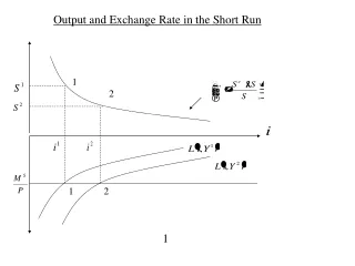
Asset Market Equilibrium • The AASchedule • It shows all the equilibrium combinations of output and the exchange rate that are consistent with the home money market and the foreign exchange market.
Asset Market Equilibrium • The AA schedule represents the asset market equilibrium • It combines the money market equilibrium with the foreign exchange equilibrium (the uncovered interest parity condition). • M/P = L(i,Y) • i = i* + (Se – S)/S
S 2' S2 i 0 i2 M P 1 M/P Asset Market Equilibrium A rise in Y 1' S1 i* + (Se-S)/S i1 L(i, Y1) L(i, Y2) 2
Asset Market Equilibrium • The equilibrium in asset markets requires: • A rise in output is related to an appreciation of the domestic currency. • The AA Schedule • It relates exchange rates and output levels that keep the asset markets in equilibrium. • It slopes downward because a rise in output causes a rise in the interest rate and a home currency appreciation.
S 1 S1 2 S2 AA Y1 Y Y2 Asset Market Equilibrium The AA Schedule
Asset Market Equilibrium • Factors that affect the AA schedule • A change in the nominal exchange rate or of output is a move along the AA schedule. • An increase in the home stock of money or a reduction in home prices shifts the AA schedule to the right. • An increase in foreign interest rate or the expected future exchange rate shifts the AA schedule to the right.
S S2 USD Rates of return 0 i2 i1 L(i, Y) M1/P M/P Asset Market Equilibrium A rise in M i* + (Se-S)/S S1 M2/P
S AA2 AA1 Y Asset Market Equilibrium A rise in M S2 S1 Y
The Short-Run Equilibrium • The short-run equilibrium brings equilibrium simultaneously to both the output and asset markets.
S DD S AA Y Y The Short-Run Equilibrium
The Short-Run Equilibrium • Reaching the short-run equilibrium. • The asset markets always reacts more rapidly. • So, we first must move toward the AA schedule. • The goods market is sticky (from sticky prices), and reacts more slowly.
S DD S2 2 S3 3 1 S1 AA Y1 Y The Short-Run Equilibrium Reaching the Equilibrium
The Short-Run Equilibrium • Reaching the short-run equilibrium • At point 2, the foreign exchange market is out of equilibrium. S is so high thati> i*+(Se-S)/S. • There is an excess demand for home currency. • So, S jumps down toward the AA schedule.
The Short-Run Equilibrium • At point 3, the goods market is out of equilibrium. S is so high that Q = SP*/P is above its equilibrium level. • This generates an excess demand for home goods. • In response, the home economy ups Y and reduces S, to reduce the excess demand. So, S and Y move along the AA schedule slowly toward the DD schedule
Temporary Policy Changes • Monetary policy • Policy instrument is the stock of money supplied. • Fiscal policy • Policy instrument is either taxes or government expenditures.
Temporary Policy Changes • Temporary Policy Changes • These policies have no effects on the expectations of future exchange rates. • We expect these changes to be temporary, and to have no effect on the long-run expected exchange rate. • So, we only worry about the short run, because we go back to the initial equilibrium. • For the following analysis, we assume that the different scenario involve no responses of foreign macroeconomic policies.
Temporary Policy Changes • A Temporary Increase in Money Supply • The Money Market • For fixed prices, the increase in the stock of money generates an excess supply of money. This reduces the home interest rate. • The expansionary monetary policy also raises output, which increases money demand. The effect, however, is small. It slightly diminishes the reduction in the home interest rate.
Temporary Policy Changes • The Foreign Exchange Market • The lower interest rate makes foreign investment more attractive. This generate an excess demand of foreign currency. The result is that the foreign currency appreciates (or the home currency depreciates). • This is a shift of the AA schedule to the right.
Temporary Policy Changes • The Goods Market • The appreciation of the foreign currency raises the real exchange rate (the price of a foreign basket of goods). This creates an excess demand for home goods: the home current account improves and pushes output up. • This is a slide along the DD schedule. • In the long run: • The initial equilibrium is restored.
S DD 2 S2 1 S1 AA1 AA2 Y1 Y2 Y Temporary Policy Changes A Temporary Monetary Expansion
Temporary Policy Changes • A Temporary Increase in Government Expenditures • In the short run: • The Goods Market • The increase in expenditures raises output. • This is a right shift of the DD schedule. • The ensuing reduction in the nominal exchange rate lowers the real exchange rate, which generates a deterioration of the current account. This small effects slightly diminishes the increase in output
Temporary Policy Changes • The Money Market • For fixed prices, the higher output raises the demand for money and the home interest rate. • The Foreign Exchange Market • The higher interest rate makes foreign investment less attractive. The result is that the foreign currency depreciates. • This is a slide along the AA schedule.
S DD1 DD2 1 S1 2 S2 AA Y1 Y Y2 Temporary Policy Changes A Temporary Increase in Government Expenditures
Temporary Policy Changes • The Business Cycle • Temporary fiscal and monetary policies can be used to neutralize the effects of outside disturbances that create recessions.
Temporary Policy Changes • For example, consider a temporary fall in world demand for home goods. • The fall in world demand creates a deterioration of the home current account at current real exchange rate. This shifts the DD schedule to the left, which lowers output and raises the exchange rate. • A temporary fiscal expansion (rise in G) would simply move the DD schedule back to its original position. This restores both output and the exchange rate. • A temporary monetary expansion would shift the AA schedule to the right. This restores output, but raises further raises the exchange rate.
S DD2 DD1 S3 3 2 S2 AA2 1 S1 AA1 Y2 Y Yf Temporary Policy Changes Countercyclical Policies: A fall in world demand
Temporary Policy Changes • For example, consider a temporary rise in money demand. • The rise in money demand raises the home interest rate, which generates an appreciation of the home currency and a reduction of home output (via a deterioration in the current account). This shifts the AA schedule to the left. • A temporary monetary expansion would shift the AA schedule back to its original position, and restores both output and the exchange rate. • A temporary fiscal expansion (rise in G) would shift the DD schedule to the right. This restores output, but further reduces the exchange rate.
S DD1 DD2 S1 1 2 S2 AA1 3 S3 AA2 Y2 Y Yf Temporary Policy Changes Countercyclical Policies: A rise in money demand