Download
1 / 62
620 likes | 770 Vues
18. Output, Exchange Rates, and Macroeconomic Policies in the Short Run. Prepared by: Fernando Quijano Dickinson State University. Introduction.

E N D
18 Output, Exchange Rates, and Macroeconomic Policies in the Short Run Prepared by:Fernando Quijano Dickinson State University
Introduction • To gain a more complete understanding of how an open economy works, we now extend our theory and explore what happens when exchange rates and output fluctuate in the short run. • We examine how macroeconomic aggregates (including output, income, consumption, investment, and the trade balance) in response to shocks in an open economy. • Recall that Y = GDP = C + I + G + TB • Our goal is to build a model that explains the relationships among all the major macroeconomic variables in an open economy in the short run. • One key lesson we learn in this chapter is that the feasibility and effectiveness of macroeconomic policies depend crucially on the type of exchange rate regime in operation.
1 Demand in the Open Economy Preliminaries and Assumptions • For our purposes, the foreign economy can be thought of as “the rest of the world” (ROW). The key assumptions we make are as follows: • Because we are examining the short run, we assume that home and foreign price levels, P and P*, are fixed due to price stickiness. As a result of price stickiness, expected inflation is fixed at zero, πe= 0. If prices are fixed, all quantities can be viewed as both real and nominal quantities in the short run because there is no inflation. • We assume that government spending G and taxes T are fixed at some constant level, which are subject to policy change. − − − − −
1 Demand in the Open Economy Preliminaries and Assumptions • We assume that conditions in the foreign economy such as foreign output Y* and the foreign interest rate i* are fixed and taken as given. Our main interest is in the equilibrium and fluctuations in the home economy. • We assume that income Y is equivalent to output: that is, gross domestic product (GDP) equals gross national disposable income (GNDI). • We further assume that net factor income from abroad (NFIA) and net unilateral transfers (NUT) are zero, which implies that the current account (CA) equals the trade balance (TB). − −
1 Demand in the Open Economy Consumption • The simplest model of aggregate private consumption relates household consumption C to disposable income Yd. • This equation is known as the Keynesian consumption function. • Marginal Effects The slope of the consumption function is called the marginal propensity to consume (MPC). We can also define the marginal propensity to save (MPS) as 1 − MPC.
1 Demand in the Open Economy Consumption FIGURE 18-1 The Consumption Function The consumption function relates private consumption, C, to disposable income, Y − T. The slope of the function is the marginal propensity to consume, MPC. ⎯
1 Demand in the Open Economy Investment • The firm’s borrowing cost is the expected real interest rate re, which equals the nominal interest rate iminus the expected rate of inflation πe: re= i− πe. • Since expected inflation is zero, the expected real interest rate equals the nominal interest rate, re= i. • Investment I is a decreasing function of the real interest rate; that is, investment falls as the real interest rate rises. • Remember that this is true only because when expected inflation is zero, the real interest rate equals the nominal interest rate.
1 Demand in the Open Economy Investment FIGURE 18-2 The Investment Function The investment function relates the quantity of investment, I, to the level of the expected real interest rate, which equals the nominal interest rate, i, when (as assumed in this chapter) the expected rate of inflation, πe, is zero. The investment function slopes downward: as the real cost of borrowing falls, more investment projects are profitable.
1 Demand in the Open Economy The Government • We will assume that the government’s role is simple. It collects an amount T of taxes from private households and spends an amount G on government consumption of goods and services. • Excluded from this concept are large sums involved in government transfer programs, such as social security, medical care, or unemployment benefit systems. • In the unlikely event that G = T exactly, we say that the government has a balanced budget. If T > G, the government is said to be running a budget surplus (of size T − G); if G > T, a budget deficit (of size G − T or, equivalently, a negative surplus of T − G). • Government purchases = G = GTaxes = T = T. − −
1 Demand in the Open Economy The Trade Balance • The Role of the Real Exchange Rate In the aggregate, when spending patterns change in response to changes in the real exchange rate, we say that there is expenditure switching from foreign purchases to domestic purchases. • If Home’s exchange rate is E, the Home price level is P (fixed in the short run), and the Foreign price level is P*(also fixed in the short run), then the real exchange rate q of Home is defined as q = EP*/P. • We expect the trade balance of the home country to be an increasing function of the home country’s real exchange rate. That is, as the home country’s real exchange rate rises (depreciates), it will export more and import less, and the trade balance rises. − − − −
1 Demand in the Open Economy The Trade Balance • The Role of Income Levels • We expect an increase in home income to be associated with an increase in home imports and a fall in the home country’s trade balance. • We expect an increase in rest of the world income to be associated with an increase in home exports and a rise in the home country’s trade balance. • The trade balance is, therefore, a function of three variables:
1 Demand in the Open Economy The Trade Balance FIGURE 18-3 (1 of 2) The Trade Balance and the Real Exchange Rate The trade balance is an increasing function of the real exchange rate, EP*/P. When there is a real depreciation (a rise in q), foreign goods become more expensive relative to home goods, and we expect the trade balance to increase as exports rise and imports fall (a rise in TB). ⎯ ⎯
1 Demand in the Open Economy The Trade Balance FIGURE 18-3 (2 of 2) The Trade Balance and the Real Exchange Rate (continued) The trade balance may also depend on income. If home income levels rise, then some of the increase in income may be spent on the consumption of imports. For example, if home income rises from Y1 to Y2, then the trade balance will decrease, whatever the level of the real exchange rate, and the trade balance function will shift down.
1 Demand in the Open Economy The Trade Balance Marginal Effects Once More We refer to MPCFas the marginal propensity to consume foreign imports. Let MPCH> 0 be the marginal propensity to consume home goods. By assumption MPC= MPCH+ MPCF. For example, if MPCF= 0.10 and MPCH= 0.65, then MPC = 0.75; for every extra dollar of disposable income, home consumers spend 75 cents, 10 cents on imported foreign goods and 65 cents on home goods (and they save 25 cents).
APPLICATION The Trade Balance and the Real Exchange Rate FIGURE 18-4 The Real Exchange Rate and the Trade Balance: United States, 1975–2006 Does the real exchange rate affect the trade balance in the way we have assumed? The data show that the U.S. trade balance is correlated with the U.S. real effective exchange rate index. Because the trade balance also depends on changes in U.S. and rest of the world disposable income (and other factors), it may respond with a lag to changes in the real exchange rate, so the correlation is not perfect (as seen in the years 2000–2006).
APPLICATION The Trade Balance and the Real Exchange Rate Barriers to Expenditure Switching: Pass-Through and the J Curve FIGURE 18-5 (2 of 2) The J Curve (continued) However, home imports now cost more due to the depreciation. Thus, the value of imports, IM, would actually rise after a depreciation, causing the trade balance TB = EX − IM to fall. Only after some time would exports rise and imports fall, allowing the trade balance to rise relative to its pre-depreciation level. The path traced by the trade balance during this process looks vaguely like a letter J.
1 Demand in the Open Economy Exogenous Changes in Demand FIGURE 18-6 (1 of 3) Exogenous Shocks to Consumption, Investment, and the Trade Balance (a) When households decide to consume more at any given level of disposable income, the consumption function shifts up.
1 Demand in the Open Economy Exogenous Changes in Demand FIGURE 18-6 (2 of 3) Exogenous Shocks to Consumption, Investment, and the Trade Balance (continued) (b) When firms decide to invest more at any given level of the interest rate, the investment function shifts right.
1 Demand in the Open Economy Exogenous Changes in Demand FIGURE 18-6 (3 of 3) Exogenous Shocks to Consumption, Investment, and the Trade Balance (continued) (c) When the trade balance increases at any given level of the real exchange rate, the trade balance function shifts up.
2 Goods Market Equilibrium: The Keynesian Cross Supply and Demand Given our assumption that the current account equals the trade balance, gross national income Y equals GDP: Aggregate demand, or just “demand,” consists of all the possible sources of demand for this supply of output. Substituting we have The goods market equilibrium condition is
2 Goods Market Equilibrium: The Keynesian Cross Determinants of Demand FIGURE 18-7 (a) (1 of 2) Panel (a): The Goods Market Equilibrium and the Keynesian Cross Equilibrium is where demand, D, equals real output or income, Y. In this diagram, equilibrium is a point 1, at an income or output level of Y1. The goods market will adjust toward this equilibrium.
2 Goods Market Equilibrium: The Keynesian Cross Determinants of Demand FIGURE 18-7 (a) (2 of 2) Panel (a): The Goods Market Equilibrium and the Keynesian Cross(continued) At point 2, the output level is Y2 and demand, D, exceeds supply, Y; as inventories fall, firms expand production and output rises toward Y1. At point 3, the output level is Y3 and supply Y exceeds demand; as inventories rise, firms cut production and output falls toward Y1.
2 Goods Market Equilibrium: The Keynesian Cross Determinants of Demand FIGURE 18-7 (b) Panel (b): Shifts in Demand The goods market is initially in equilibrium at point 1, at which demand and supply both equal Y1. An increase in demand, D, at all levels of real output, Y, shifts the demand curve up from D1 to D2. Equilibrium shifts to point 2, where demand and supply are higher and both equal Y2. Such an increase in demand could result from changes in one or more of the components of demand: C, I, G, or TB.
2 Goods Market Equilibrium: The Keynesian Cross Factors That Shift the Demand Curve The opposite changes lead to a decrease in demand and shift the demand curve in.
3 Goods and Forex Market Equilibria: Deriving the IS Curve Equilibrium in Two Markets • A general equilibrium requires equilibrium in all markets—that is, equilibrium in the goods market, the money market, and the forex market. • The IS curve shows combinations of output Y and the interest rate i for which the goods and forex markets are in equilibrium. Forex Market Recap Uncovered interest parity (UIP) (Equation (18-3)) :
Exchange Rates and Interest Rates in the Short Run:UIP and FX Market Equilibrium TABLE 15-1 Interest Rates, Exchange Rates, Expected Returns, and FX Market Equilibrium: A Numerical Example The foreign exchange (FX) market is in equilibrium when the domestic and foreign returns are equal. In this example, the dollar interest rate is 5%, the euro interest rate is 3%, and the expected future exchange rate (one year ahead) is = 1.224 $/€. The equilibrium is highlighted in bold type, where both returns are 5% in annual dollar terms. Figure 12-2 plots the domestic and foreign returns (columns 1 and 6) against the spot exchange rate (column 3). Figures are rounded in this table.
Exchange Rates and Interest Rates in the Short Run:UIP and FX Market Equilibrium Equilibrium in the FX Market: An Example FIGURE 15-2 FX Market Equilibrium: A Numerical Example The returns calculated in Table 15-1 are plotted in this figure. The dollar interest rate is 5%, the euro interest rate is 3%, and the expected future exchange rate is 1.224 $/€. The foreign exchange market is in equilibrium at point 1, where the domestic returns DR and expected foreign returns FR are equal at 5% and the spot exchange rate is 1.20 $/€.
3 Goods and Forex Market Equilibria: Deriving the IS Curve Deriving the IS Curve FIGURE 18-8 (1 of 3) Deriving the IS Curve The Keynesian cross is in panel (a), IS curve in panel (b), and forex (FX) market in panel (c). The economy starts in equilibrium with output, Y1; interest rate, i1; and exchange rate, E1. Consider the effect of a decrease in the interest rate from i1 to i2, all else equal. In panel (c), a lower interest rate causes a depreciation; equilibrium moves from 1′ to 2′.
3 Goods and Forex Market Equilibria: Deriving the IS Curve Equilibrium in Two Markets FIGURE 18-8 (2 of 3) Deriving the IS Curve (continued) A lower interest rate boosts investment and a depreciation boosts the trade balance. In panel (a), demand shifts up from D1 to D2, equilibrium from 1” to 2”, output from Y1 to Y2.
3 Goods and Forex Market Equilibria: Deriving the IS Curve Deriving the IS Curve FIGURE 18-8 (3 of 3) Deriving the IS Curve (continued) In panel (b), we go from point 1 to point 2. The IS curve is thus traced out, a downward-sloping relationship between the interest rate and output. When the interest rate falls from i1 to i2, output rises from Y1 to Y2. The IS curve describes all combinations of i and Y consistent with goods and FX market equilibria in panels (a) and (c).
3 Goods and Forex Market Equilibria: Deriving the IS Curve Deriving the IS Curve • One important observation is in order: • In an open economy, lower interest rates stimulate demand through the traditional closed-economy investment channel and through the trade balance. • The trade balance effect occurs because lower interest rates cause a nominal depreciation (in the short run, it is also a real depreciation), which stimulates external demand via the trade balance. • The IS curve is downward-sloping. It illustrates the negative relationship between the interest rate i and output Y.
3 Goods and Forex Market Equilibria: Deriving the IS Curve Factors That Shift the IS Curve FIGURE 18-9 (1 of 2) Exogenous Shifts in Demand Cause the IS Curve to Shift In the Keynesian cross in panel (a), when the interest rate is held constant at i1 , an exogenous increase in demand (due to other factors) causes the demand curve to shift up from D1 to D2 as shown, all else equal. This moves the equilibrium from 1” to 2”, raising output from Y1 to Y2.
3 Goods and Forex Market Equilibria: Deriving the IS Curve Factors That Shift the IS Curve FIGURE 18-9 (2 of 2) Exogenous Shifts in Demand Cause the IS Curve to Shift (continued) In the IS diagram in panel (b), output has risen, with no change in the interest rate. The IS curve has therefore shifted right from IS1 to IS2. The nominal interest rate and hence the exchange rate are unchanged in this example, as seen in panel (c).
3 Goods and Forex Market Equilibria: Deriving the IS Curve Summing Up the IS Curve Factors That Shift the IS Curve The opposite changes lead to a decrease in demand and shift the demand curve down and the IS curve to the left.
4 Money Market Equilibrium: Deriving the LM Curve • In this section, we derive a set of combinations of Y and i that ensures equilibrium in the money market, a concept that can be represented graphically as the LM curve. Money Market Recap • In the short-run, the price level is assumed to be sticky at a level P, and the money market is in equilibrium when the demand for real money balances L(i)Y equals the real money supply M/P: – – (18-2)
4 Money Market Equilibrium: Deriving the LM Curve Deriving the LM Curve FIGURE 18-10 (1 of 2) Deriving the LM Curve If there is an increase in real income or output from Y1 to Y2 in panel (b), the effect in the money market in panel (a) is to shift the demand for real money balances to the right, all else equal. If the real supply of money, MS, is held fixed at M/P, then the interest rate rises from i1 to i2 and money market equilibrium moves from point 1′ to point 2′. ⎯
4 Money Market Equilibrium: Deriving the LM Curve Deriving the LM Curve FIGURE 18-10 (2 of 2) Deriving the LM Curve (continued) The relationship thus described between the interest rate and income, all else equal, is known as the LM curve and is depicted in panel (b) by the movement from point 1 to point 2. The LM curve is upward-sloping: when the output level rises from Y1 to Y2, the interest rate rises from i1 to i2. The LM curve describes all combinations of i and Y that are consistent with money market equilibrium in panel (a).
4 Money Market Equilibrium: Deriving the LM Curve Factors That Shift the LM Curve FIGURE 18-11 (1 of 2) Change in the Money Supply Shifts the LM Curve In the money market, shown in panel (a), we hold fixed the level of real income or output, Y, and hence real money demand, MD. All else equal, we show the effect of an increase in money supply from M1 to M2. The real money supply curve moves out from MS1 to MS2. This moves the equilibrium from 1′ to 2′, lowering the interest rate from i1 to i2.
4 Money Market Equilibrium: Deriving the LM Curve Factors That Shift the LM Curve FIGURE 18-11 (2 of 2) Change in the Money Supply Shifts the LM Curve (continued) In the LM diagram, shown in panel (b), the interest rate has fallen, with no change in the level of income or output, so the economy moves from point 1 to point 2. The LM curve has therefore shift down from LM1 to LM2.
4 Money Market Equilibrium: Deriving the LM Curve Summing Up the LM Curve Factors That Shift the LM Curve
5 The Short-Run IS-LM-FX Model of an Open Economy FIGURE 18-12 (1 of 2) Equilibrium in the IS-LM-FX Model In panel (a), the IS and LM curves are both drawn. The goods and forex markets are in equilibrium when the economy is on the IS curve. The money market is in equilibrium when the economy is on the LM curve. Both markets are in equilibrium if and only if the economy is at point 1, the unique point of intersection of IS and LM.
5 The Short-Run IS-LM-FX Model of an Open Economy FIGURE 18-13 (2 of 2) Equilibrium in the IS-LM-FX Model (continued) In panel (b), the forex (FX) market is shown. The domestic return, DR, in the forex market equals the money market interest rate. Equilibrium is at point 1′ where the foreign return FR equals domestic return, i.
5 The Short-Run IS-LM-FX Model of an Open Economy Macroeconomic Policies in the Short Run • We focus on the two main policy actions: changes in monetary policy, implemented through changes in the money supply, and changes in fiscal policy, involving changes in government spending or taxes. • The key assumptions of this section are as follows. • The economy begins in a state of long-run equilibrium. We then consider policy changes in the home economy, assuming that conditions in the foreign economy (i.e., the rest of the world) are unchanged. • The home economy is subject to the usual short-run assumption of a sticky price level at home and abroad. • Furthermore, we assume that the forex market operates freely and unrestricted by capital controls and that the exchange rate is determined by market forces.
5 The Short-Run IS-LM-FX Model of an Open Economy Monetary Policy under Floating Exchange Rates FIGURE 18-13 (1 of 2) Monetary Policy under Floating Exchange Rates In panel (a) in the IS-LM diagram, the goods and money markets are initially in equilibrium at point 1. The interest rate in the money market is also the domestic return, DR1, that prevails in the forex market. In panel (b), the forex market is initially in equilibrium at point 1′. A temporary monetary expansion that increases the money supply from M1 to M2 would shift the LM curve down in panel (a) from LM1 to LM2, causing the interest rate to fall from i1 to i2. DR falls from DR1 to DR2.
5 The Short-Run IS-LM-FX Model of an Open Economy Monetary Policy under Floating Exchange Rates FIGURE 18-13 (2 of 2) Monetary Policy under Floating Exchange Rates (continued) In panel (b), the lower interest rate implies that the exchange rate must depreciate, rising from E1 to E2. As the interest rate falls (increasing investment, I) and the exchange rate depreciates (increasing the trade balance), demand increases, which corresponds to the move down the IS curve from point 1 to point 2’. Output expands from Y1 to Y2. The new equilibrium corresponds to points 2 and 2′.
5 The Short-Run IS-LM-FX Model of an Open Economy Monetary Policy under Floating Exchange Rates To sum up: a temporary monetary expansion under floating exchange rates is effective in combating economic downturns by boosting output. It raises output at home, lowers the interest rate, and causes a depreciation of the exchange rate. What happens to the trade balance cannot be predicted with certainty.
5 The Short-Run IS-LM-FX Model of an Open Economy Monetary Policy under Fixed Exchange Rates FIGURE 18-14 (1 of 2) Monetary Policy under Fixed Exchange Rates In panel (a) in the IS-LM diagram, the goods and money markets are initially in equilibrium at point 1. In panel (b), the forex market is initially in equilibrium at point 1′. A temporary monetary expansion that increases the money supply from M1 to M2 would shift the LM curve down in panel (a).
5 The Short-Run IS-LM-FX Model of an Open Economy Monetary Policy under Fixed Exchange Rates FIGURE 18-14 (2 of 2) Monetary Policy under Fixed Exchange Rates (continued) In panel (b), the lower interest rate would imply that the exchange rate must depreciate, rising from E1to E2. This depreciation is inconsistent with the pegged exchange rate, so the policy makers cannot move LM in this way. They must leave the money supply equal to M1. Implication: under a fixed exchange rate, autonomous monetary policy is not an option. ⎯ ⎯
5 The Short-Run IS-LM-FX Model of an Open Economy Monetary Policy under Fixed Exchange Rates To sum up: monetary policy under fixed exchange rates is impossible to undertake. Fixing the exchange rate means giving up monetary policy autonomy. Countries cannot simultaneously allow capital mobility, maintain fixed exchange rates, and pursue an autonomous monetary policy.
5 The Short-Run IS-LM-FX Model of an Open Economy Fiscal Policy under Floating Exchange Rates FIGURE 18-15 (1 of 3) Fiscal Policy under Floating Exchange Rates In panel (a) in the IS-LM diagram, the goods and money markets are initially in equilibrium at point 1. The interest rate in the money market is also the domestic return, DR1, that prevails in the forex market. In panel (b), the forex market is initially in equilibrium at point 1′.