Major analytical/theoretical techniques
330 likes | 353 Vues
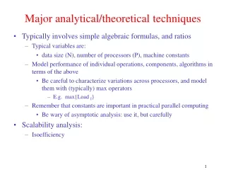
Major analytical/theoretical techniques. Typically involves simple algebraic formulas, and ratios Typical variables are: data size (N), number of processors (P), machine constants Model performance of individual operations, components, algorithms in terms of the above

Major analytical/theoretical techniques
E N D
Presentation Transcript
Major analytical/theoretical techniques • Typically involves simple algebraic formulas, and ratios • Typical variables are: • data size (N), number of processors (P), machine constants • Model performance of individual operations, components, algorithms in terms of the above • Be careful to characterize variations across processors, and model them with (typically) max operators • E.g. max{Load I} • Remember that constants are important in practical parallel computing • Be wary of asymptotic analysis: use it, but carefully • Scalability analysis: • Isoefficiency
Scalability • The Program should scale up to use a large number of processors. • But what does that mean? • An individual simulation isn’t truly scalable • Better definition of scalability: • If I double the number of processors, I should be able to retain parallel efficiency by increasing the problem size
Equal efficiency curves Problem size processors Isoefficiency • Quantify scalability • How much increase in problem size is needed to retain the same efficiency on a larger machine? • Efficiency : Seq. Time/ (P · Parallel Time) • parallel time = computation + communication + idle • One way of analyzing scalability: • Isoefficiency: • Equation for equal-efficiency curves • Use η(p,N) = η(x.p, y.N) to get this equation • If no solution: the problem is not scalable • in the sense defined by isoefficiency
Simplified Communication Basics • Communication cost, for a n-byte message • = ά + n β • Incurred by each processor (sender and receiver) • Later, we will use a more sophisticated analysis • Take into account different components involved: • Co-processors, network contention, • bandwidth, bisection bandwidth
Introduction to recurring applications • We will use these applications as examples • Jacobi Relaxation • Classic finite-stencil-on-regular-grid code • Molecular Dynamics for biomolecules • Interacting 3D points with short- and long-range forces • Rocket Simulation • Multiple interacting physics modules • Cosmology / Tree-codes • Barnes-hut-like fast trees
Jacobi Relaxation Sequential pseudoCode: Decomposition by: While (maxError > Threshold) { Re-apply Boundary conditions maxError = 0; for i = 0 to N-1 { for j = 0 to N-1 { B[i,j] = 0.2(A[i,j] + A[I,j-1] +A[I,j+1] + A[I+1, j] + A[I-1,j]) ; if (|B[i,j]- A[i,j]| > maxError) maxError = |B[i,j]- A[i,j]| } } swap B and A } Row Blocks Or Column
Row decomposition Computation per proc: A.N*N/P Communication Ratio: Efficiency: Isoefficiency: Block decomposition Commputation per proc: A.NxN/P Communication: Ratio Efficiency Isoefficiency Isoefficiency of Jacobi Realaxation
Molecular Dynamics in NAMD • Collection of [charged] atoms, with bonds • Newtonian mechanics • Thousands of atoms (1,000 - 500,000) • 1 femtosecond time-step, millions needed! • At each time-step • Calculate forces on each atom • Bonds: • Non-bonded: electrostatic and van der Waal’s • Short-distance: every timestep • Long-distance: every 4 timesteps using PME (3D FFT) • Multiple Time Stepping • Calculate velocities and advance positions Collaboration with K. Schulten, R. Skeel, and coworkers
Traditional Approaches: non isoefficient • Replicated Data: • All atom coordinates stored on each processor • Communication/Computation ratio: P log P • Partition the Atoms array across processors • Nearby atoms may not be on the same processor • C/C ratio: O(P) • Distribute force matrix to processors • Matrix is sparse, non uniform, • C/C Ratio: sqrt(P) Not Scalable
Spatial Decomposition • Atoms distributed to cubes based on their location • Size of each cube : • Just a bit larger than cut-off radius • Communicate only with neighbors • Work: for each pair of nbr objects • C/C ratio: O(1) • However: • Load Imbalance • Limited Parallelism Cells, Cubes or“Patches”
Object Based Parallelization for MD: Force Decomposition + Spatial Deomp. • Now, we have many objects to load balance: • Each diamond can be assigned to any proc. • Number of diamonds (3D): • 14·Number of Patches
A C B Bond Forces • Multiple types of forces: • Bonds(2), Angles(3), Dihedrals (4), .. • Luckily, each involves atoms in neighboring patches only • Straightforward implementation: • Send message to all neighbors, • receive forces from them • 26*2 messages per patch! • Instead, we do: • Send to (7) upstream nbrs • Each force calculated at one patch
Virtualized Approach to implementation: using Charm++ 192 + 144 VPs 700 VPs 30,000 VPs These 30,000+ Virtual Processors (VPs) are mapped to real processors by charm runtime system
Rocket Simulation • Dynamic, coupled physics simulation in 3D • Finite-element solids on unstructured tet mesh • Finite-volume fluids on structured hex mesh • Coupling every timestep via a least-squares data transfer • Challenges: • Multiple modules • Dynamic behavior: burning surface, mesh adaptation Robert Fielder, Center for Simulation of Advanced Rockets Collaboration with M. Heath, P. Geubelle, others
Computational Cosmology • Here, we focus on n-body aspects of it • N particles (1 to 100 million), in a periodic box • Move under gravitation • Organized in a tree (oct, binary (k-d), ..) • Processors may request particles from specific nodes of the tree • Initialization and postmortem: • Particles are read (say in parallel) • Must distribute them to processor roughly equally • Must form the tree at runtime • Initially and after each step (or a few steps) • Issues: • Load balancing, fine-grained communication, tolerating communication latencies. • More complex versions may do multiple-time stepping Collaboration with T. Quinn, Y. Staedel, others
Causes of performance loss • If each processor is rated at k MFLOPS, and there are p processors, why don’t we see k•p MFLOPS performance? • Several causes, • Each must be understood separately, first • But they interact with each other in complex ways • Solution to one problem may create another • One problem may mask another, which manifests itself under other conditions (e.g. increased p).
Performance Issues • Algorithmic overhead • Speculative Loss • Sequential Performance • Critical Paths • Bottlenecks • Communication Performance • Overhead and grainsize • Too many messages • Global Synchronization • Load imbalance
Why Aren’t Applications Scalable? • Algorithmic overhead • Some things just take more effort to do in parallel • Example: Parallel Prefix (Scan) • Speculative Loss • Do A and B in parallel, but B is ultimately not needed • Load Imbalance • Makes all processor wait for the “slowest” one • Dynamic behavior • Communication overhead • Spending increasing proportion of time on communication • Critical Paths: • Dependencies between computations spread across processors • Bottlenecks: • One processor holds things up
Algorithmic Overhead • Sometimes, we have to use an algorithm with higher operation count in order to parallelize an algorithm • Either the best sequential algorithm doesn’t parallelize at all • Or, it doesn’t parallelize well (e.g. not scalable) • What to do? • Choose algorithmic variants that minimize overhead • Use two level algorithms • Examples: • Parallel Prefix (Scan) • Game Tree Search
Parallel Prefix • Given array A[0..N-1], produce B[N], such that B[k] is the sum of all elements of A upto A[k] B[0] = A[0]; for (I=1; I<N; I++) B[I] = B[I-1]+A[I]; Data dependency from iteration to iteration. How can this be parallelized at all? Theoreticians to the rescue: they came up with a clever algorithm.
Parallel prefix : recursive doubling N Data Items P Processors N=P Log P Phases P additions in each phase P log P ops Completes in O(P) time
Parallel Prefix: Engineering • Issue : N >> P • Recursive doubling : Naïve implementation • Operation count: log(N) . N • A better implementation: well-engineered: • Take blocking of data into account • Each processor calculate its sum, then • Participates in a parallel algorithm (with P numbers) • to get sum to its left, and then adds to all its elements • N + log(P) +N: • Only doubling of operation Count • What did we do? • Same algorithm, better parallelization/engineering
Parallelization overhead: summary of advice • Explore alternative algorithms • Unless the algorithmic overhead is inevitable! • Don’t take algorithms that say “We use f(N) processors to solve a problem of size N” as they are. • Use Clyde Kruskal’s metric • Performance results must be in terms of • N data items, P processors • Reformulate accordingly
Algorithmic overhead: Game Tree Search • Game Trees for 2-person, zero-sum games (Chess) • Bad Sequential Algorithm: • Min-Max tree • Good Sequential algorithm: Evaluate using a-b search • Relies on left-to-right evaluation (dependency!) • Not parallel! • Prunes a large number of nodes
Algorithmic overhead: Game Tree Search • A (simple) solution: • Use min-max at top level of trees • Below a certain threshold (simple: depth), • use sequential a-b • Other variations: • Use prioritized tree generation at high levels, with Left-to-Right bias • Use a-b at top! Firing only essential leaves as subtasks • Useful for small # of processors • Or, relax “essential” in interesting ways
Speculative Loss: Branch and Bound • Problem and parallelization via objects • B&B leads to a search tree, with pruning • Tree is naturally parallel structure, but… • Speculative loss: • Number of tree nodes processed increases with procs • Solution: Scalable Prioritized load balancing • Memory balancing • Good Speedup on 512 processors • 1024 processor NCUBE, in 1990+ • Lessons: • Importance of priorities • Need to work with application experts! Sinha and Kale, 1992, Prioritized Load Balancing
Critical Paths • What: Long chain of dependence • that holds a computation step up • Diagnostic: • Performance scales upto P processors, after which is stagnates to a (relatively) fixed value • That by itself may have other causes…. • Solution: • Eliminate long chains if possible • Shorten chains by removing work from critical path
Bottlenecks • How to detect: • One processor A is busy while others wait • And there is a data dependency on the result produced by A • Typical situations: • Everyone sends data to one processor, which computes some function and sends result to everyone. • Master-slave: one processor assigning job in response to requests • Solution techniques: • Typically, solved by using a spanning tree based collection mechanism • Hierarchical schemes for master slave • What makes it hard: • Program may not show ill effects for a long time • Eventually someone runs it on a large machine, where it shows up
Bootlenecks master With More Slave processors With Few Slave processors Master overhead: V Slave time: S Number of processors: P If (P<S/V): speedup = P (approx.) If (P>S/V) speedup = S/V
Communication Operations • Kinds of communication operations: • Point-to-point • Synchronization • Barriers, Scalar Reductions • Vector reductions • Data size is significant • Broadcasts • Short (Signals) • Large • Global (Collective) operations • All-to-all operations, gather, scatter
Communication Basics: Point-to-point Sending processor Sending Co-processor Network Receiving co-processor Receiving processor Elan-3 cards on alphaservers (TCS): Of 2.3 μs “put” time 1.0 : proc/PCI 1.0 : elan card 0.2: switch 0.1 Cable Each component has a per-message cost, and per byte cost