Download
1 / 36
360 likes | 401 Vues
Understand the runoff components in hydrology - overland flow, interflow, base flow - analyzing hydrographs and flow-mass curves for stream characteristics. Learn about drainage basins, water years, flow-duration curve construction, and flow mass curve calculations.

E N D
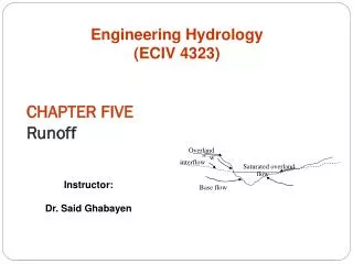
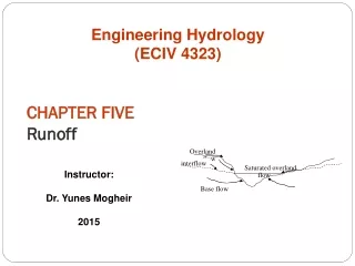
Overland flow interflow Saturated overland flow Base flow CHAPTER FIVE Runoff Engineering Hydrology (ECIV 4323) Instructor: Dr. Yunes Mogheir 2015
Runoff Parts • Runoff normally applies to flow over a surface • Overland flow: is the surface runoff from tracts of land (or sheet flow) before it reaches a defined channel . • Stream flow is used to describe the drainage after it reaches a defined channel • Drainage basins, watersheds, sub-basins, catchments:Defined by the total area contributing to a specific point. This point varies with the objectives of the project.
Stream Flow Components: • Direct precipitation on the channel (typically incorporated into total basin area) • Overland flow: when soil moisture storage and depression storage are filled “excess” rainfall generates overland flow. • Interflow: all rainfall that infiltrates does not reach saturated zone (ground water). Under certain conditions infiltrated moisture can travel through shallow soil horizons. Usually only significant for highly permeable soils. • Baseflow: contribution to stream flow from groundwater
5.2 Hydrograph • Streamflow in terms of discharge vs time is represented by the hydrograph. • Hydrograph components thus become, • surface runoff • interflow • baseflow • direct precipitation • Direct Runoff: all moisture that reaches the stream channel without first entering zone of saturation (overland flow + interflow) • Streamflow = direct runoff + baseflow
Water Year In annual runoff studies it is advantageous to consider a water year beginning from the time when the precipitation exceeds the average evaporation losses.
5.3 Runoff characteristics of streams • Perennial Stream (Fig 5.2) • A stream which always carries some flow. It is always fed from groundwater base flow. Even during dry seasons the water table will be above the bed of the stream. Stream is always fed from groundwater base flow
An intermittent stream (Fig. 5.3) • Stream is fed from groundwater base only in the wet season. During the wet season the water table is above the stream bed. During dry seasons the water table drops to a level lower than that of the stream bed; and therefore the stream dries up. Stream is fed from Groundwater base only in the wet season
An ephemeral steam(Fig 5.4) • No contribution from groundwater (base flow) to the stream (most rivers in arid zones) No contribution from groundwater (base flow) to the stream (most rivers in arid zones)
5.5 Flow-Duration curve • Is a plot of discharge against the percentage of time the flow was equaled or exceeded (Discharge-Frequency curve) • Step of construction the curve • Stream flow discharge is arranged in decreasing order. • Use class interval if we have very large number of records (example 5.8) • Use plotting position to compute the probability of equal or exceeded. • m= order number of discharge (class value) • N= number of data • Pp= percentage probability • Plot the discharge Q against Pp (Fig 5.8) • Or semi-log or log-log paper (Fig 5.10)
5.5 Flow-Duration curve • The flow duration curve represents the cumulative frequency distribution • The percentage probability of time that flow magnitude in average year is equal or greater • Q50 = 100 m3/s • Example 5.8
Example 5.8 The daily flows of a river for three consecutive years are shown in the table below. For convenience the discharges are shown in class intervals and the number of days the flow belonged to the class is shown. Calculate the 50 and 75% dependable flows for the river
5.6 Flow mass curve • The flow-mass curve is a plot of cumulative discharge against time plotted in sequential order • The flow-mass curve integral curve (summation curve) of the hydrograph • See figure 5.11
… Flow mass curve • Unit is volume million m3 or m3/s day, cm over a catchment area • Slope of the mass curve =dv/dt =Q = flow rate • Average flow rate in the time between tm and tn • Slope of line AB is the average over whole period records
Calculation of storage volume • Assume there is a reservoir on a stream where FM curve is shown in Fig 5.9 and it is full at the beginning of a dry period, i.e. when the inflow rate is less than the withdrawal (demand) rate, the storage (S) of the reservoir • VD =demand volume (withdrawal) • VS = supply volume (Inflow) • The storage “S” is the maximum cumulative deficiency in any dry season. It is obtained as the maximum difference in the ordinate between mass curves of supply & demand. • If there are two dry periods, the minimum storage volume required is the largest of S1 and S2 (Fig. 5.9)
… Calculation of storage volume • i.e. The minimum storage volume required by a reservoir is the largest value of S • Refer to Figure 5.11 • CD is drawn tangential to the first part of curve • Qd slope of CD is a constant rate of withdrawal from the reservoir • The lowest capacity is reached at E where EF is tangential at E • S1: the water volume needed as storage to meet the maximum demand (reservoir is full) • S2: is for C’D’ • Then the minimum reservoir storage required is the largest storage S2>S1
Example 5.9 The following table gives the mean monthly flows in a river during 1981. Calculate the minimum storage required to maintain a demand rate of 40 m3/s.
… example 5.9 The actual number of days in the month are used in calculating the monthly flow volume. Volumes are calculated in units of cumec. day (= 8.64×10⁴ m3)
Refer to Example 5.9 • Compute the monthly flow volume by using the actual days in each month • Compute the accumulated volume in (cumec – day) or in m3. • Plot the flow mass curve (accumulated flow volume and time) • Draw a tangential line with slope of 40 m3/s • Slope = y/x y=x(slope) • y= 60.8 days x 40 =2432 cumec-day • To draw the demand line, the number of days in a month can be taken as 30.4 days.
Calculation of storage volume • Refer to Example 5.9 • Flow mass curve (Figure 5.12) • Draw parallel line to AB in the valley point A’B’ • Vertical value S1 is the storage required to maintain the demand • From figure 5.12 2100 m3/s.day • Solve Example 5.10
Example 5.10 Work out the example 5.9 through arithmetic calculation without the use of the mass curve
Calculation of maintainable demand • The storage volume is given. Your job is now to determine the maximum demand that can be maintained by this given storage volume. • Fig. 5.13: • Tangents are drawn from the ridges and valleys of the mass curves at various slopes (since we still don’t know the demand!). • The demand line that requires just the given storage is the proper demand that can be sustained by the reservoir in that dry period. • Similar demand lines are drawn at other valleys. • The smallest of the various demand rates thus is the maximum solid demand that can be sustained by the given storage
Variable demand • In practice the demand rate varies with time to meet various end uses (such as irrigation, power and water supply needs, etc.) • A mass curve of demand is prepared and superposed on the flow-mass curve.
In the analysis of problems related to reservoirs it is necessary to account for evaporation, leakage, and other losses from the reservoir. • These losses can either be included in demand rates or deducted from inflow rates. If you used the second method, the mass curve may have negative slopes at some points. • Solve Example 5.12