Chapter 9 : Differential Analysis of Fluid Flow

1. PTT 204/3APPLIED FLUID MECHANICSSEM 2 (2012/2013) Chapter 9: Differential Analysis of Fluid Flow

2. Objectives • Understand how the differentialequation of conservation ofmass is derivedand applied • Calculate the stream functionand pressure field, and plotstreamlines for a knownvelocity field • Obtain analytical solutionsof the equations of motionfor simple flow fields

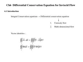
3. 9–1 ■ INTRODUCTION The control volume technique is useful when we are interested in the overall features of a flow, such as mass flow rate into and out of the control volume or net forces applied to bodies. Differential analysis, on the other hand, involves application of differential equations of fluid motion to any and every point in the flow field over a region called the flow domain. Boundary conditionsfor the variables must be specified at all boundaries of the flow domain, including inlets, outlets, and walls. If the flow is unsteady, we must march our solution along in time as the flow field changes. (a) In control volume analysis, the interior of the control volume is treated like a black box, but (b) in differential analysis, all the details of the flow are solved at every point within the flow domain.

4. 9–2 ■ CONSERVATION OF MASS—THE CONTINUITY EQUATION The net rate of change of mass within the control volume is equal to the rate at which mass flows into the control volume minus the rate at which mass flows out of the control volume. To derive a differential conservation equation, we imagine shrinking a control volume to infinitesimal size.

5. Derivation Using the Divergence Theorem The quickest and most straightforward way to derive the differential form of conservation of mass is to apply the divergence theorem (Gauss’s theorem). This equation is the compressible form of the continuity equation since we have not assumed incompressible flow. It is valid at any point in the flow domain.

6. Derivation Using an Infinitesimal Control Volume At locations away from the center of the box, we use a Taylor series expansionabout the center of the box. A small box-shaped control volume centered at point P is used for derivation of the differential equation for conservation of mass in Cartesian coordinates; the blue dots indicate the center of each face.

7. The mass flow rate through a surface is equal to VnA. The inflow or outflow of mass through each face of the differential control volume; the blue dots indicate the center of each face.

8. The divergence operation in Cartesian and cylindrical coordinates.

9. Alternative Form of the Continuity Equation As a material element moves through a flow field, its density changes according to Eq. 9–10.

10. Continuity Equation in Cylindrical Coordinates Velocity components and unit vectors in cylindrical coordinates: (a) two-dimensional flow in the xy- or r-plane, (b) three-dimensional flow.

11. Special Cases of the Continuity Equation Special Case 1: Steady Compressible Flow

12. Special Case 2: Incompressible Flow The disturbance from an explosion is not felt until the shock wave reaches the observer.

14. The continuity equation can be used to find a missing velocity component.

16. 9–3 ■ THE STREAM FUNCTION The Stream Function in Cartesian Coordinates Incompressible, two-dimensional stream function in Cartesian coordinates: stream function  There are several definitions of the stream function, depending on the type of flow under consideration as well as the coordinate system being used.

17. Curves of constant stream function represent streamlines of the flow. Curves of constant  are streamlines of the flow.

19. Streamlines for the velocity field of Example 9–8; the value of constant  is indicated for each streamline, and velocity vectors are shown at four locations.

22. Streamlines for the velocity field of Example 9–9; the value of constant  is indicated for each streamline.

23. The difference in the value of  from one streamline to another is equal to the volume flow rate per unit width between the two streamlines. (a) Control volume bounded by streamlines 1 and 2 and slices A and B in the xy-plane; (b) magnified view of the region around infinitesimal length ds.

24. The value of  increases to the left of the direction of flow in the xy-plane. Illustration of the “left-side convention.” In the xy-plane, the value of the stream function always increases to the left of the flow direction. In the figure, the stream function increases to the left of the flow direction, regardless of how much the flow twists and turns. When the streamlines are far apart (lower right of figure), the magnitude of velocity (the fluid speed) in that vicinity is small relative to the speed in locations where the streamlines are close together (middle region). This is because as the streamlines converge, the cross-sectional area between them decreases, and the velocity must increase to maintain the flow rate between the streamlines.

25. The Stream Function in Cylindrical Coordinates Flow over an axisymmetric body in cylindrical coordinates with rotational symmetry about the z-axis; neither the geometry nor the velocity field depend on , and u = 0.

26. Streamlines for the velocity field of Example 9–12, with K = 10 m2/s and C = 0; the value of constant  is indicated for several streamlines.

28. The Compressible Stream Function

29. 9–5 ■ THE NAVIER–STOKES EQUATION Introduction ij, called the viscous stress tensoror the deviatoric stress tensor Mechanical pressure is the mean normal stress acting inwardly on a fluid element. For fluids at rest, the only stress on a fluid element is the hydrostatic pressure, which always acts inward and normal to any surface.

30. Newtonian versus Non-Newtonian Fluids Rheology:The study of the deformation of flowing fluids. Newtonian fluids:Fluids for which the shear stress is linearly proportional to the shear strain rate. Non-Newtonian fluids:Fluids for which the shear stress is not linearly related to the shear strain rate. Viscoelastic:A fluid that returns (either fully or partially) to its original shape after the applied stress is released. Some non-Newtonian fluids are called 1) Shear thinning fluidsor pseudoplasticfluids: The more the fluid is sheared, the less viscous it becomes. 2) Shear thickening fluidsor dilatant fluids: The more the fluid is sheared, the more viscous it becomes. Rheological behavior of fluids—shear stress as a function of shear strain rate. In some fluids a finite stress called the yield stressis required before the fluid begins to flow at all; such fluids are called Bingham plastic fluids.

31. Derivation of the Navier–Stokes Equation for Incompressible, Isothermal Flow The incompressible flow approximation implies constant density, and the isothermal approximation implies constant viscosity.

32. The Laplacian operator, shown here in both Cartesian and cylindrical coordinates, appears in the viscous term of the incompressible Navier–Stokes equation.

33. The Navier–Stokes equation is an unsteady, nonlinear, secondorder, partial differential equation. Equation 9–60 has four unknowns (three velocity components and pressure), yet it represents only three equations (three components since it is a vector equation). Obviously we need another equation to make the problem solvable. The fourth equation is the incompressible continuity equation (Eq. 9–16). The Navier–Stokes equation is the cornerstone of fluid mechanics.

34. Continuity and Navier–Stokes Equations in Cartesian Coordinates

35. Continuity and Navier–Stokes Equations in Cylindrical Coordinates

36. An alternative form for the first two viscous terms in the r- and -components of the Navier–Stokes equation.

37. Summary • Introduction • Conservation of mass-The continuity equation • Derivation Using the Divergence Theorem • Derivation Using an Infinitesimal Control Volume • Alternative Form of the Continuity Equation • Continuity Equation in Cylindrical Coordinates • Special Cases of the Continuity Equation • The stream function • The Stream Function in Cartesian Coordinates • The Stream Function in Cylindrical Coordinates • The Compressible Stream Function

38. The Navier-Stokes equation • Introduction • Newtonian versus Non-Newtonian Fluids • Derivation of the Navier–Stokes Equation for Incompressible, Isothermal Flow • Continuity and Navier–Stokes Equations in Cartesian Coordinates • Continuity and Navier–Stokes Equations in Cylindrical Coordinates

39. Thank You…