Chapter 8: Flow in Pipes
Chapter 8: Flow in Pipes. ME 331 – Fluid Dynamics Spring 2008. Objectives. Have a deeper understanding of laminar and turbulent flow in pipes and the analysis of fully developed flow

Chapter 8: Flow in Pipes
E N D
Presentation Transcript
Chapter 8: Flow in Pipes ME 331 – Fluid Dynamics Spring 2008
Objectives • Have a deeper understanding of laminar and turbulent flow in pipes and the analysis of fully developed flow • Calculate the major and minor losses associated with pipe flow in piping networks and determine the pumping power requirements • Understand the different velocity and flow rate measurement techniques and learn their advantages and disadvantages
Introduction • Average velocity in a pipe • Recall - because of the no-slip condition, the velocity at the walls of a pipe or duct flow is zero • We are often interested only in Vavg, which we usually call just V (drop the subscript for convenience) • Keep in mind that the no-slip condition causes shear stress and friction along the pipe walls Friction force of wall on fluid
Introduction • For pipes of constant diameter and incompressible flow • Vavg stays the same down the pipe, even if the velocity profile changes • Why? Conservation of Mass Vavg Vavg same same same
Introduction • For pipes with variable diameter, m is still the same due to conservation of mass, but V1 ≠ V2 D1 D2 m V1 V2 m 2 1
Laminar and Turbulent Flows • Critical Reynolds number (Recr) for flow in a round pipe Re < 2300 laminar 2300 ≤ Re ≤ 4000 transitional Re > 4000 turbulent • Note that these values are approximate. • For a given application, Recr depends upon • Pipe roughness • Vibrations • Upstream fluctuations, disturbances (valves, elbows, etc. that may disturb the flow) Definition of Reynolds number
Laminar and Turbulent Flows • For non-round pipes, define the hydraulic diameter Dh = 4Ac/P Ac= cross-section area P = wetted perimeter • Example: open channel Ac= 0.15 * 0.4 = 0.06m2 P = 0.15 + 0.15 + 0.5 = 0.8m Don’t count free surface, since it does not contribute to friction along pipe walls! Dh = 4Ac/P = 4*0.06/0.8 = 0.3m What does it mean? This channel flow is equivalent to a round pipe of diameter 0.3m (approximately).
The Entrance Region • Consider a round pipe of diameter D. The flow can be laminar or turbulent. In either case, the profile develops downstream over several diameters called the entry lengthLh. Lh/D is a function of Re. Lh
Fully Developed Pipe Flow • Comparison of laminar and turbulent flow There are some major differences between laminar and turbulent fully developed pipe flows Laminar • Can solve exactly (Chapter 9) • Flow is steady • Velocity profile is parabolic • Pipe roughness not important It turns out that Vavg = 1/2Umax and u(r)= 2Vavg(1 - r2/R2)
Instantaneousprofiles Fully Developed Pipe Flow Turbulent • Cannot solve exactly (too complex) • Flow is unsteady (3D swirling eddies), but it is steady in the mean • Mean velocity profile is fuller (shape more like a top-hat profile, with very sharp slope at the wall) • Pipe roughness is very important • Vavg 85% of Umax (depends on Re a bit) • No analytical solution, but there are some good semi-empirical expressions that approximate the velocity profile shape. See text Logarithmic law (Eq. 8-46) Power law (Eq. 8-49)
Laminar Turbulent slope slope w w Fully Developed Pipe Flow Wall-shear stress • Recall, for simple shear flows u=u(y), we had = du/dy • In fully developed pipe flow, it turns out that = du/dr w = shear stress at the wall, acting on the fluid w,turb > w,lam
w Take CV inside the pipe wall P1 P2 V L 2 1 Fully Developed Pipe Flow Pressure drop • There is a direct connection between the pressure drop in a pipe and the shear stress at the wall • Consider a horizontal pipe, fully developed, and incompressible flow • Let’s apply conservation of mass, momentum, and energy to this CV (good review problem!)
Fully Developed Pipe Flow Pressure drop • Conservation of Mass • Conservation of x-momentum Terms cancel since 1 = 2 and V1 = V2
Fully Developed Pipe Flow Pressure drop • Thus, x-momentum reduces to • Energy equation (in head form) or cancel (horizontal pipe) Velocity terms cancel again because V1 = V2, and 1 = 2 (shape not changing) hL = irreversible head loss & it is felt as a pressuredrop in the pipe
Fully Developed Pipe Flow Friction Factor • From momentum CV analysis • From energy CV analysis • Equating the two gives • To predict head loss, we need to be able to calculate w. How? • Laminar flow: solve exactly • Turbulent flow: rely on empirical data (experiments) • In either case, we can benefit from dimensional analysis!
Fully Developed Pipe Flow Friction Factor • w = func( V, , D, ) = average roughness of the inside wall of the pipe • -analysis gives
Fully Developed Pipe Flow Friction Factor • Now go back to equation for hL and substitute f for w • Our problem is now reduced to solving for Darcy friction factor f • Recall • Therefore • Laminar flow: f = 64/Re (exact) • Turbulent flow: Use charts or empirical equations (Moody Chart, a famous plot of f vs. Re and /D, See Fig. A-12, p. 898 in text) But for laminar flow, roughness does not affect the flow unless it is huge
Fully Developed Pipe Flow Friction Factor • Moody chart was developed for circular pipes, but can be used for non-circular pipes using hydraulic diameter • Colebrook equation is a curve-fit of the data which is convenient for computations (e.g., using EES) • Both Moody chart and Colebrook equation are accurate to ±15% due to roughness size, experimental error, curve fitting of data, etc. Implicit equation for f which can be solved using the root-finding algorithm in EES
Types of Fluid Flow Problems • In design and analysis of piping systems, 3 problem types are encountered • Determine p (or hL) given L, D, V (or flow rate) Can be solved directly using Moody chart and Colebrook equation • Determine V, given L, D, p • Determine D, given L, p, V (or flow rate) • Types 2 and 3 are common engineering design problems, i.e., selection of pipe diameters to minimize construction and pumping costs • However, iterative approach required since both V and D are in the Reynolds number.
Types of Fluid Flow Problems • Explicit relations have been developed which eliminate iteration. They are useful for quick, direct calculation, but introduce an additional 2% error
Minor Losses • Piping systems include fittings, valves, bends, elbows, tees, inlets, exits, enlargements, and contractions. • These components interrupt the smooth flow of fluid and cause additional losses because of flow separation and mixing • We introduce a relation for the minor losses associated with these components • KL is the loss coefficient. • Is different for each component. • Is assumed to be independent of Re. • Typically provided by manufacturer or generic table (e.g., Table 8-4 in text).
i pipe sections j components Minor Losses • Total head loss in a system is comprised of major losses (in the pipe sections) and the minor losses (in the components) • If the piping system has constant diameter
Piping Networks and Pump Selection • Two general types of networks • Pipes in series • Volume flow rate is constant • Head loss is the summation of parts • Pipes in parallel • Volume flow rate is the sum of the components • Pressure loss across all branches is the same
Piping Networks and Pump Selection • For parallel pipes, perform CV analysis between points A and B • Since p is the same for all branches, head loss in all branches is the same
Piping Networks and Pump Selection • Head loss relationship between branches allows the following ratios to be developed • Real pipe systems result in a system of non-linear equations. Very easy to solve with EES! • Note: the analogy with electrical circuits should be obvious • Flow flow rate (VA) : current (I) • Pressure gradient (p) : electrical potential (V) • Head loss (hL): resistance (R), however hL is very nonlinear
Piping Networks and Pump Selection • When a piping system involves pumps and/or turbines, pump and turbine head must be included in the energy equation • The useful head of the pump (hpump,u) or the head extracted by the turbine (hturbine,e), are functions of volume flow rate, i.e., they are not constants. • Operating point of system is where the system is in balance, e.g., where pump head is equal to the head losses.
Pump and systems curves • Supply curve for hpump,u: determine experimentally by manufacturer. When using EES, it is easy to build in functional relationship for hpump,u. • System curve determined from analysis of fluid dynamics equations • Operating point is the intersection of supply and demand curves • If peak efficiency is far from operating point, pump is wrong for that application.