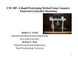
CNC-RP: A Rapid Prototyping Method Using Computer Numerical Controlled Machining

1. CNC-RP: A Rapid Prototyping Method Using Computer Numerical Controlled Machining Matthew C. Frank Industrial and Manufacturing Engineering Iowa State University Richard A. Wysk Industrial and Systems Engineering North Carolina State University

2. Agenda What is RP? Limitations of RP Economics of RP New directions in RP Observations and conclusions 2

3. Prototyping is critically important during product/process design Reduce time to market Early detection of errors Assist concurrent manufacturing engineering Prototypes are used to convey a products’: Form Fit Function Prototype building can be a time-consuming process requiring a highly skilled craftsperson Time spent testing prototypes is valuable Time spent constructing them is not… “Rapid Prototyping” (RP) methods have emerged (Solid Freeform Fabrication, Additive Manufacturing, Layered Manufacturing) Introduction Need for model accuracy increases 3

4. Stereolithography (SLA) Stereolithography is a common rapid manufacturing and rapid prototyping technology for producing parts with high accuracy and good surface finish. A device that performs stereolithography is called an SLA or Stereolithography Apparatus. Stereolithography is an additive fabrication process utilizing a vat of liquid UV-curablephotopolymer "resin" and a UVlaser to build parts a layer at a time. On each layer, the laser beam traces a part cross-section pattern on the surface of the liquid resin.

5. Selective Laser Sintering (SLS) SLS can produce parts from a relatively wide range of commercially available powder materials, including polymers (nylon, also glass-filled or with other fillers, and polystyrene), metals (steel, titanium, alloy mixtures, and composites) and green sand. The physical process can be full melting, partial melting, or liquid-phase sintering. And, depending on the material, up to 100% density can be achieved with material properties comparable to those from conventional manufacturing methods. In many cases large numbers of parts can be packed within the powder bed, allowing very high productivity.

6. Fused Deposition Modeling (FDM) • Fused deposition modeling, which is often referred to by its initials FDM, is a type of rapid prototyping or rapid manufacturing (RP) technology commonly used within engineering design. The technology was developed by S. Scott Crump in the late 1980s and was commercialized in 1990. The FDM technology is marketed commercially by Stratasys Inc. • Like most other RP processes (such as 3D Printing and stereolithography) FDM works on an "additive" principle by laying down material in layers. A plastic filament or metal wire is unwound from a coil and supplies material to an extrusion nozzle which can turn on and off the flow. The nozzle is heated to melt the material and can be moved in both horizontal and vertical directions by a numerically controlled mechanism, directly controlled by a Computer Aided Design software package. In a similar manner to stereolithography, the model is built up from layers as the material hardens immediately after extrusion from the nozzle. • Several materials are available with different trade-offs between strength and temperature. As well as Acrylonitrile butadiene styrene (ABS) polymer, the FDM technology can also be used with polycarbonates, polycaprolactone, and waxes. A "water-soluble" material can be used for making temporary supports while manufacturing is in progress. Marketed under the name WaterWorks by Stratasys this soluble support material is actually dissolved in a heated sodium hydroxide solution with the assistance of ultrasonic agitation.

7. Laminated Object Manufacturing (LOM) Laminated Object Manufacturing (LOM) is a rapid prototyping system developed by Helisys Inc. (Cubic Technologies is now the successor organization of Helisys) In it, layers of adhesive-coated paper, plastic, or metal laminates are successively glued together and cut to shape with a knife or laser cutter.

8. Electron Beam Melting (EBM) • Electron Beam Melting (EBM) is a type of rapid prototyping for metal parts. It is often classified as a rapid manufacturing method. The technology manufactures parts by melting metal powder layer per layer with an electron beam in a high vacuum. Unlike some metal sintering techniques, the parts are fully solid, void-free, and extremely strong. Electron Beam Melting is also referred to as Electron Beam Machining. • High speed electrons .5-.8 times the speed of light are bombarded on the surface of the work material generating enough heat to melt the surface of the part and cause the material to locally vaporize. EBM does require a vacuum, meaning that the workpiece is limited in size to the vacuum used. The surface finish on the part is much better than that of other manufacturing processes. EBM can be used on metals, non-metals, ceramics, and composites.

9. Types of RP Systems

10. Time and Cost to machine

11. Material cost In most cases this is independent of the number of parts 11

12. t =(t + t ) j j + t + t + t j P m c i setup L/UL j t setup j t j t m t c t i Production time per piece / nbt the time required for setup for an operation (load fixture, retrieve tooling , etc.) the time required to load and unload a product for feature operation j (chuck, fixture, etc..) L/UL the machining/processing time for feature j tool change time/part idle time due to scheduling control nbt number of parts per batch

13. / / + + C n C = t n C C p p mo t setup p/t p/t • The product cost can be expressed as: Production cost per piece, Cp

14. where Cmo is the cost of machine and operator/hour Ct is the perishable tooling cost np/t is the number of pieces that can be produced per tool Csetup is the setup resource cost for the part (fixture, jig, steady-rest, etc)

15. Problem Introduction physical models • Rapid Prototyping? • Technology for producing accurate parts directly from CAD models in a few hours with little need for human intervention. • Pham, et al, 1997 • Prototype? • A first full-scale and usually functional form of a new type or design of a construction (as an airplane) • Webster’s, 1998 • Model? • A representation in relief or 3 dimensions in plaster, papier-mache, wood, plastic, or other material of a surface or solid • Webster’s, 1986 How can we automatically create toolpath and fixture plans for CNC?

16. Engineering cost CE = Ced / nt + Cpc / nt + Cpd / nb total parts total parts parts in a batch 16

17. Manufacturing cost • One time costs • Process planning and design • Fixture engineering and fabrication • Set up cost (Cset) • Cost to set up a process • Processing cost (Cpsc) • Cost of processing a part • Production cost (Cpdc) • Cost of tooling and perishables 17

18. Manufacturing cost CM = Cone / nt + Cset / nb + Cpsc + Cpdc // ntool Total partsparts in a batch each part tool cost by parts/tool 18

19. So how can engineering costs be reduced for CNC machining? Machine cost Fixture cost Process planning cost

20. CNC-RP Method: A part is machined on a 3-Axis mill with a rotary indexer and tailstock using layer-based toolpaths from numerous orientations about an axis of rotation.

21. STEPS TO CREATE A PART ( MT. Bike Suspension Component)

22. STEPS TO CREATE A PART ( MT. Bike Suspension Component)

23. Process/fixture planning time: Minutes Processing time ~20 hours Material: Steel Layer depth: 0.001” (0.025mm)

24. PROCESSING STEPS (Side View) Machine the visible surfaces from each of a set of orientations using layer-based toolpaths ROTATE to next orientation MACHINE ROTATE The number of rotations required to machine a model is dependent on its geometric complexity MACHINE ROTATE MACHINE REMOVE model at sacrificial supports

25. Methodology • Creation of complex parts using a series of thin layers (slices) of 3-axis toolpaths generated at numerous orientations rotated about an axis of the part • Toolpath planning based on “layering” methods used by other RP systems • “Slice” represents visible cross-sectional area to be machined about (subtractive) rather than actual cross section to be deposited (additive) • Slice thickness is the depth of cut for the 2½-D toolpaths • Tool used is a flat end mill cutter with equal flute and shank diameter (or shank diameter < flute diameter) • Stock material will be cylindrical, therefore toolpath z-zero location will be same for all orientations

26. Flat end mill cutter “Staircase” effect Region not visible from current orientation Set of visible slices from current orientation Toolpath planning using this approach is done with ease in current CAM software (MasterCAM rough surface pocketing) Methodology (cont.)

27. Methodology (cont.) • Fixturing accomplished through temporary feature(s) (cylinders) appended to the solid model prior to toolpath planning • Cylinders attached to solid model along the axis of rotation • Incrementally created during machining operation as the model is rotated • Model remains secured to stock material then removed (similar to support structures in current RP methods)

28. Rapid Prototyping • Basics: • Solid model (CAD) is converted to STL format • Facetted representation where surface is approximated by triangles • Intersect the STL model with parallel planes to create cross sections • Create each cross section, adding on top of preceding one CAD (ProE) STL “slicing” operation 2-D cross section

29. Model material Support material Build Platform Rapid Prototyping • Fixtures are created in-process (Sacrificial Supports) • Secure model to the build platform • Support overhanging features • Remove fixture materials in post-process step FDM Model with/without supports

30. RP versus CNC Machining Functional prototypes? • RP processes are very flexible and very capable • However: • RP processes rely on specialized materials • Limited accuracy in some cases • CNC Machining is: • Subtractive process • Accurate • Capable of using many common manufacturing materials • CNC Machining is NOT: • Automated • Easily usable except by highly skilled technicians • CNC machining cannot create all parts • No hollow parts • No severely undercut features • The time consuming tasks of process and fixture planning are major factors which prohibit CNC machining from being used as a Rapid Prototyping Process • Wang et al, 1999

31. Previous Work • Chen and Song, 1991 • Layer based machining for prototyping • Machined layers using robotic arm/machine tool • Layers laminated in a stack • Merz, et al, 1994 • Shape Deposition Manufacturing • Additive/Subtractive Process • Walczyk and Hardt, 1998; Vouezelaud et al, 1992 • Rapid tooling • Laminated machining for dies • Lennings, 2000 • Deskproto software • CNC machining planner • Processes similar to a mill/turn operation

32. Motivation • RP processes are almost completely automated “turnkey” operations • User does not have to be skilled technician • Process planning is simplified by layer-based approach • Fixtures are created in process • The approach to CNC-RP will have to relax many of the traditional constraints • Efficient machining is not a major driver (Traditional feeds/speeds not used) • Not feature-based (Not necessary to machine entire feature in one setup orientation) • Surface finish not as critical (Allow staircase effect) • Goal of this research is to develop a method for CNC rapid prototyping such that: • Toolpath planning, sequencing, tool sizing is automated • Fixture design is created in-process, flexible, and allows access to almost all surfaces • Setups/orientation automatically calculated, executed • No collision problems

33. Toolpath layers at 0º orientation Toolpath layers at 180º orientation z y x z y x z z y y Methodology • Overview: • Visible surfaces of the part are machined from each orientation about an axis of rotation • Long, small diameter flat end tool with equal flute and shank diameter used. • Sacrificial supports (temporary features) added to the solid model and created in-process • Begin with round stock material, clamped between two opposing chucks • Example:

34. Research Problems • Setup/Orientation • How many rotations (setup orientations) about the axis of rotation are required? • Where are they? • Toolpath planning • For each orientation, how can we automatically generate toolpaths? • What diameter and length tools should be used? • In what order should the toolpaths be executed? • Fixture planning • How can we automatically generate sacrificial supports? • What diameter and length should they be?

35. Determining the number of rotations • A problem of tool accessibility • Approximated as a problem of visibility (line of sight) • A Visibility map is generated via a layer-based approach • Tool access is restricted to directions in the slice plane (2D problem) • Goal is to generate the data necessary to determine a minimum set of rotations required to machine the entire surface Set of segments on a slice visible from one tool access direction

36. Approaches to 2D visibility mapping • Shortest Euclidean paths - Lee and Preparata, 1984 • Convex ropes - Peshkin and Sanderson, 1986 • 2D visibility cones - Stewart, 1999 • Issues: • Computing S.E.P.s/VCs for polygons with holes • Granularity of STL files, may need to add collinear points to polygon segments • Would need to retriangulate

37. Solution approach • Visibility for each polygonal chain is determined by calculating the polar angle range that each segment of the chain can be seen. • Since there can be multiple chains on each slice, we must consider the visibility blocked by all other chains. (b) Visibility for the segment= [Θa,Θb,], [Θc,Θd,] (a) Visibility for the segment= [Θa,Θb,]

38. Pi+1 not visible Pi-1 Pi+1 P: , S: LCHP RCHP Pi RCHP LCHP Pi Step one: Visibility with respect to own chain • We have a polygon P and its convex hull S • For any point Pinot on S, the visible range can be found by investigating points from the adjacent CCW convex hull point to the adjacent CW convex hull point • These points will be denoted the “left” and “right” convex hull points of Pi, LCHP(Pi) and RCHP(Pi), respectively. • It is only necessary to calculate the polar angles from Pi to the points in the set [LCHP, RCHP], excluding Pi. • The set is divided into, S1 and S2 where:

39. V(Pi): [43.82 ,121.31] S1 S2 V(Pi) Pi • The visible range for a point is bounded by the minimum polar angle from Pi to points in S1 and the maximum polar angle from Pi to points in S2. • This is the visible range for the point Piwith respect to the boundary of its own chain, and is denoted V(Pi). • Where:

40. RVv LVv LVu RVu u-1 v+1 v u • Consider the segment defined by points in P, u and v, where: • u: Pi and v: Pi+1 • The intersection of visibility ranges for the points u and v and the 180º range above the segment define a feasible range of polar angles in which the segment could be reached. • The sets S1 and S2 are redefined: • The ends of the visibility range are:

41. LV I1 u I2 v I2 u v I1 LV RV (a) (b) RV RV LV RV LV I2 I2 I1 I1 v u u v (c) (d) Problem Surfaces (a) RV is outside of the 180º range, (b) Both RV and LV are out of the 180º range, (c) No visibility due to overlapping, (d) Visibility to the entire segment is not possible since RV > LV.

42. Step two: Visibility blocked by all other chains on the slice • V( )j* is the visibility with respect to the chain j on which resides, denoted j*. • For all obstacle chains , the polar range blocked by the chain is denoted VB( )j. • The set of visible ranges for the segment is defined: • Visibility blocked to the segment is the union of the visibility blocked by chain j to point u and the visibility blocked by chain j to point v, intersected with the 180º range above segment • The set of angles blocked to the segment where: • The set of angles blocked to points u and v where:

43. LBu RBv LBv RBu v u • Considering the condition that blocked visibility is only for blockage in the 180º range above the segment, it can easily be seen that the set: • RBu is simply the minimum polar angle from u to all points on the blocker chain • LBv is the maximum polar angle from v to all points on Pj, where Pj is the set of points for the blocker chain.

44. Recall: • For each segment the collection of visible ranges given in polar angle about the axis of rotation: where: rMAX = n • From the data in [VIS] we can formulate a set corresponding to the segments visible from a given angle. The Minimum Set Cover problem: Given: A collection of subsets Θsof a finite set SEG(the set of all segments) Solution: A set cover for SEG, i.e., a subset S’S such that every element in SEG belongs to at least one member of Θs for .

45. 49º 140º 228º 320º Implementation/Results • Algorithm implemented in C • Computation times on a 2.0GHz Pentium 4 • Set cover problem solved as integer linear program using LINDO: The “Jack”…

46. z z y z y x y x y z x x Results (cont) Cell phone face plate… Turbine…

47. Toolpath Planning • Layer based toolpaths • Machine visible surfaces from approach direction • 2½-D pocketing, easily generated using current CAM software (MasterCAM, rough surface pocketing) • A gouge-free approach, given flute and shank diameter are same (or shank < flute) • Investigated as a rough machining approach - Balasubramanium, 1999 • Can approach finish machining using very small depths of cut • We assume that tool length, not diameter will be active constraint • To avoid collision, tool length > maximum swept diameter of part (Same as stock diameter) • Tool diameter chosen as smallest available for required length (not conventional tools)

48. d Depth of cut(max) = -Ds Where Ds= Stock Diameter Toolpath Planning • Stock diameter/Tool length can be found from slice data used in VISI algorithm • For each slice, find diameter of the set of points • Set stock diameter to MAX • Ds = MAXDIAM(CHP(slice points)) for all slices k • Set tool length to diameter of the stock Lt = Ds • Toolpath sequencing is a significant problem • Need to avoid “thin web” conditions • Can occur during one toolpath or from successive toolpaths Ds = Ds + 2d (1) Lt = Ds + d (2)

49. (3) Toolpath Planning • Thin material conditions resulting from thru-pocket part geometry: • For each successive toolpath planned in sequence, undesirable orientations to be avoided:

50. Toolpath Planning • Preparatory toolpath sequence to avoid thin material conditions • Removes bulk of stock material prior to processing remainder of toolpaths • Choose from orientations in the solution set, or add new Model Remaining stock material *Preparatory passes adhere to condition: (3)