NUMERICAL INTEGRATION AND DIFFERENTIATION Student Notes
NUMERICAL INTEGRATION AND DIFFERENTIATION Student Notes. ENGR 351 Numerical Methods for Engineers Southern Illinois University Carbondale College of Engineering Dr. L.R. Chevalier Dr. B.A. DeVantier. Specific Study Objectives. Understand the derivation of the Newton-Cotes formulas

NUMERICAL INTEGRATION AND DIFFERENTIATION Student Notes
E N D
Presentation Transcript
NUMERICAL INTEGRATION AND DIFFERENTIATION Student Notes ENGR 351 Numerical Methods for Engineers Southern Illinois University Carbondale College of Engineering Dr. L.R. Chevalier Dr. B.A. DeVantier
Specific Study Objectives • Understand the derivation of the Newton-Cotes formulas • Recognize that the trapezoidal and Simpson’s 1/3 and 3/8 rules represent the areas of 1st, 2nd, and 3rd order polynomials • Be able to choose the “best” among these formulas for any particular problem
Specific Study Objectives • Recognize the difference between open and closed integration formulas • Understand the theoretical basis of Richardson extrapolation and how it is applied • Recognize why both Romberg integration and Gauss quadrature have utility when integrating equations (as opposed to tabular or discrete data)
Specific Study Objectives • Understand basic finite difference approximations • Understand the application of high-accuracy numerical-differentiation • Recognize data error on the processes of integration and differentiation
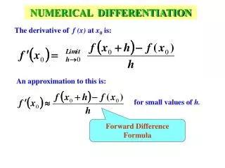
Numerical Differentiation and Integration • Calculus is the mathematics of change. • Engineers must continuously deal with systems and processes that change, making calculus an essential tool of our profession. • At the heart of calculus are the related mathematical concepts of differentiation and integration.
Differentiation • Dictionary definition of differentiate - “to mark off by differences, distinguish; ..to perceive the difference in or between” • Mathematical definition of derivative - rate of change of a dependent variable with respect to an independent variable
f(x) Dy Dx x
Integration • The inverse process of differentiation • Dictionary definition of integrate - “to bring together, as parts, into a whole; to unite; to indicate the total amount” • Mathematically, it is the total value or summation of f(x)dx over a range of x. In fact the integration symbol is actually a stylized capital S intended to signify the connection between integration and summation.
f(x) a b x
Overview • Newton-Cotes Integration Formulas • Trapezoidal rule • Simpson’s Rules • Unequal Segments • Open Integration • Integration of Equations • Romberg Integration • Gauss Quadrature • Improper Integrals
Overview • Numerical Differentiation • High accuracy formulas • Richardson’s extrapolation • Unequal spaced data • Uncertain data • Applied problems
Newton-Cotes Integration • Common numerical integration scheme • Based on the strategy of replacing a complicated function or tabulated data with some approximating function that is easy to integrate
The approximation of an integral by the area under - a first order polynomial - a second order polynomial We can also approximated the integral by using a series of polynomials applied piece wise.
An approximation of an integral by the area under straight line segments.
Newton-Cotes Formulas • Closed form - data is at the beginning and end of the limits of integration • Open form - integration limits extend beyond the range of data.
Trapezoidal Rule • First of the Newton-Cotes closed integration formulas • Corresponds to the case where the polynomial is a first order
Trapezoidal Rule A straight line can be represented as:
Trapezoidal Rule Integrate this equation. Results in the trapezoidal rule.
Trapezoidal Rule Recall the formula for computing the area of a trapezoid: (height)(average of the bases) base height base
Trapezoidal Rule The concept is the same but the trapezoid is on its side. base height height height width base
Error of the Trapezoidal Rule This indicates that is the function being integrated is linear, the trapezoidal rule will be exact. Otherwise, for section with second and higher order derivatives (that is with curvature) error can occur. A reasonable estimate ofx is the average value of b and a Guide to pronouncing Greek letters
Example Evaluate the following integral using the trapezoidal rule. Estimate the error Strategy
Strategy • Using the graph, illustrate the problem. • Isolate the function • Calculate the function at the two endpoints, a and b • Using the values of a,b, f(a), and f(b), estimate I • Estimate error
Multiple Application of the Trapezoidal Rule • Improve the accuracy by dividing the integration interval into a number of smaller segments • Apply the method to each segment • Resulting equations are called multiple-application or composite integration formulas
Multiple Application of the Trapezoidal Rule When there are n+1 equally spaced base points, we can group terms to express a general form } } width average height
} } width average height Multiple Application of the Trapezoidal Rule The average height represents a weighted average of the function values Note that the interior points are given twice the weight of the two end points
Example Evaluate the following integral using the trapezoidal rule and h = 0.1 Strategy
Strategy • Isolate the function to be solved • Determine n • Graphically evaluate the problem to be solved • Expand the governing equation • Make a table of the needed values of f(x) • Estimate the integral • Estimate the error
Simpson’s 1/3 Rule • Corresponds to the case where the function is a second order polynomial
Simpson’s 1/3 Rule • Designate a and b as x0and x2, and estimate f2(x) as a second order Lagrange polynomial
} } width average height Simpson’s 1/3 Rule • After integration and algebraic manipulation, we get the following equations
Error Single application of Trapezoidal Rule. Single application of Simpson’s 1/3 Rule
The odd points represent the middle term for each application. Hence carry the weight 4. The even points are common to adjacent applications and are counted twice. i=1 (odd) weight of 4 i=2 (even) weight of 2 f(x) x
Simpson’s 3/8 Rule • Corresponds to the case where the function is a third order polynomial
Integration of Unequal Segments • Experimental and field study data is often unevenly spaced • In previous equations we grouped the term (i.e. hi) which represented segment width.
Integration of Unequal Segments • We should also consider alternately using higher order equations if we can find data in consecutively even segments trapezoidal rule 1/3 rule trapezoidal rule 3/8 rule
Example Integrate the following using the trapezoidal rule, Simpson’s 1/3 Rule, a multiple application of the trapezoidal rule with n=2 and Simpson’s 3/8 Rule. Compare results with the analytical solution. Strategy
Strategy • Solve the problem analytically. Your error will be based on this true value • For error, use the equation for et • Isolate the function • Graphically consider the problem • Identify the governing equation for each estimate • For each method, determine n and h. Make a table of x and f(x) • Estimate the integral. Compare the results
Integration of Equations • Integration of analytical as opposed to tabular functions • Romberg Integration • Richardson’s Extrapolation • Romberg Integration Algorithm • Gauss Quadrature • Improper Integrals
Richardson’s Extrapolation Estimate the integral using two different step sizes. If h1 = h2/2 then
Example: Class Demonstration Use Richardson’s extrapolation to evaluate:
Solution Recall our previous example where we calculated the integral using a single application of the trapezoidal rule, and then a multiple application of the trapezoidal rule by dividing the interval in half.
Solution Therefore h2 = h1 / 2. We can use a special case that will be introduced later in lecture.
Solution SINGLE APPLICATION OF TRAPEZOIDAL RULE MULTIPLE APPLICATION OF TRAPEZOIDAL RULE (n=2) RICHARDSON’S EXTRAPOLATION 357% 133% 58% ....end of example
Richardson’s Extrapolation • Use two estimates of an integral to compute a third more accurate approximation • The estimate and error associated with a multiple application trapezoidal rule can be represented generally as: • I = I(h) + E(h) • where I is the exact value of the integral • I(h) is the approximation from an n-segment application • E(h) is the truncation error • h is the step size (b-a)/n
Richardson’s Extrapolation Make two separate estimates using step sizes of h1and h2. I(h1) + E(h1) = I(h2) + E(h2) Recall the error of the multiple-application of the trapezoidal rule Assume that is constant regardless of the step size