Download
1 / 16
170 likes | 267 Vues
Learn about numerical differentiation methods such as forward and backward approximation, Lagrange polynomial interpolation, and numerical quadrature for integration accuracy. Understand composite numerical integration and error analysis for accurate results.

E N D
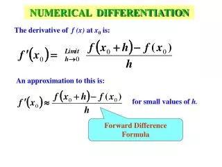
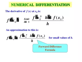
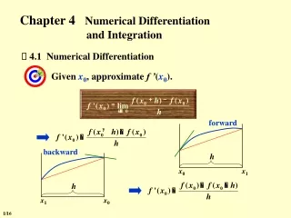
Given x0, approximatef ’(x0). + - f ( x h ) f ( x ) = 0 0 f ' ( x ) lim 0 h 0 h h h x0 x1 x1 x0 Chapter 4Numerical Differentiation and Integration 4.1 Numerical Differentiation forward backward 1/16
Chapter 4 Numerical Differentiation and Integration -- Numerical Differentiation Approximate f(x) by its Lagrange polynomial with interpolating points x0 and x0 + h. O(h) f ’(x0) = f (x) = f ’(x) = 2/16
Chapter 4 Numerical Differentiation and Integration -- Numerical Differentiation Approximate f(x) by its Lagrange polynomial with interpolating points { x0, x1, …, xn }. f ’(xj) = Note: In general, more evaluation points produce greater accuracy. On the other hand, the number of functional evaluations grows and the roundoff error increases. Hence the numerical differentiation is unstable! 3/16
Chapter 4 Numerical Differentiation and Integration -- Numerical Differentiation x–1 x0 x1 Example: Given three points x0, x0 + h, and x0 + 2h, please derive the three-point formulae for each of the points. Symmetric to formula 1, with h < 0. Five-point formulae are given on p.171 4/16
Chapter 4 Numerical Differentiation and Integration -- Numerical Differentiation Excuses for not doing homework I could only get arbitrarily close to my textbook. I couldn't actually reach it. 2 1 h [ ] = - - + + - x ( 4 ) f ( x ) f ( x h ) 2 f ( x ) f ( x h ) f ( ) 0 0 0 0 2 h 12 Approximate f ”(x0) Consider Taylor expansions of f(x0 + h) and f(x0 – h) at x0: HW: p.176-177 #7, 13 5/16
Chapter 4 Numerical Differentiation and Integration -- Elements of Numerical Integration Approximate Integrate the Lagrange interpolating polynomial of f (x) instead. Error Select a set of distinct nodes a x0 < x1 <…< xn b from [a, b]. The Lagrange polynomial is Idea Ak 4.3 Elements of Numerical Integration -- Numerical Quadrature interpolatory quadrature 6/16
Chapter 4 Numerical Differentiation and Integration -- Elements of Numerical Integration Example: Consider the linear interpolation on [a, b], we have f(x) a b f(b) f(a) Definition: The degree of accuracy, or precision, of a quadrature formula is the largest positive integer n such that the formula is exact for xk for each k = 0, 1, …, n. Please determine the precision of this formula. Solution: Consider xk for each k = 0, 1, … trapezoidal rule x0 =1: = x : = Degree of Precision = 1 x2 : 7/16
Chapter 4 Numerical Differentiation and Integration -- Elements of Numerical Integration n = 1: For equally spaced nodes: Let Cotes coefficient Note: Cotes coefficients does not depend on either f(x) or [a, b], and can be determined by n and ionly. Hence we can find these coefficients from a table. The formulae are called Newton-Cotes formulae. Trapezoidal Rule Precision = 1 8/16
Chapter 4 Numerical Differentiation and Integration -- Elements of Numerical Integration n = 2: n = 3: Simpson’s 3/8-Rule. Precision = 3, and n = 4: Cotes Rule. Precision = 5, and Theorem: For the (n+1)-point closed Newton-Cotes formula, there exists (a, b) for which if n is even and f Cn+2[a, b], and if n is odd and f Cn+1[a, b]. Simpson’s Rule Precision = 3 HW: p.195 #7, 9, 11, 13 9/16
Chapter 4 Numerical Differentiation and Integration -- Composite Numerical Integration /*MVT*/ 4.4 Composite Numerical Integration Due to the oscillatory nature of high-degree polynomials, piecewise interpolation is applied to approximate f(x) a piecewise approach that uses the low-order Newton-Cotes formulae. Composite Trapezoidal Rule: Apply Trapezoidal Rule on each [xk – 1, xk]: Oh come on, you don’t seriously consider h=(ba)/2 acceptable, do you? Don’t you forget the oscillatory nature of high- degree polynomials! Haven’t we had enough formulae? What’s up now? Why can’t you simply refine the partition if you have to be so picky? Uh-oh =Tn 10/16
Chapter 4 Numerical Differentiation and Integration -- Composite Numerical Integration 4 4 4 4 4 Note: To simplify the notation, we may let n’ = 2n. Then and Composite Simpson’s Rule: =Sn 11/16
Chapter 4 Numerical Differentiation and Integration -- Composite Numerical Integration Composite integration techniques are all stable. Example: Consider the Simpson’s Rule with n subintervals on [a, b]. Assume that f (xi) is approximated by f *(xi) such that f (xi) = f *(xi) + i for each i = 0, 1, …, n. Then the accumulated error e(h) is If | i| < for all i = 0, 1, …, n, then When we refine the partition to ensure accuracy, the increased computation will NOT increase the roundoff error. 12/16
Chapter 4 Numerical Differentiation and Integration -- Composite Numerical Integration Example: Use Trapezoidal rule and Simpson’s rule with n = 8 to approximate where where Solution: = 3.138988494 = 3.141592502 When programming we usually keep dividing the subintervals into 2 equally spaced smaller subintervals. That is, take n = 2k for k = 0, 1, … HW: p.204 #7(a)(b) Whenk = 9, T512 = 3.14159202 = 3.141592502 = S4 13/16
Chapter 4 Numerical Differentiation and Integration -- Romberg Integration ( ( ( ( ( ( ( ( ( ( 1 0 2 3 2 1 1 0 0 0 ) ) ) ) ) ) ) ) ) ) T T T T T T T T T T 2 2 1 0 1 0 0 1 0 3 Since the error of Trapezoidal rule is when we reduce the length of each subinterval into a half, T1 = T2 = S1 = T4 = S2 = C1 = T8 = S4 = C2 = R1 = 4.5 Romberg Integration Romberg sequence Solve for I : = Sn In general: < ? Romberg method: < ? < ? … … … … … … 14/16
Lab 08. Shape Roof Time Limit: 2 seconds; Points: 4 The kind of roof shown in Figure 1 is shaped from plain flat rectangular plastic board in Figure 2. Figure 1 Figure 2 The transection of the roof is a sine curve with altitude l centimeters. Given the length of the roof, your task is to calculate the length of the flat board needed to shape the roof. 15/16
Chapter 4 Numerical Differentiation and Integration -- Richardson’s Extrapolation Generate high-accuracy results while using low-order formulae - 2 T ( ) T ( h ) 1 3 h - = - a - a - 2 3 0 0 2 I h h ... 2 3 - 2 1 2 4 4.2 Richardson’s Extrapolation Suppose that for some h 0, we have a formula T0(h) that approximates an unknown I, and that the truncation error has the form: T0(h) I = 1 h + 2 h2 + 3 h3 + … Replace hby half its value, we have T0(h/2) I = 1 (h/2) + 2 (h/2)2 + 3 (h/2)3 + … Q:How to improve the accuracy from O(h) to O(h2) ? 16/16