Numerical Differentiation and Integration Methods
Learn numerical differentiation using formulas and error estimates, and numerical integration techniques like Trapezoidal Rule and Simpson’s Rule for approximating unknown functions. Understand the concept behind Riemann sum and composite methods.

Numerical Differentiation and Integration Methods
E N D
Presentation Transcript
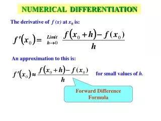
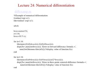
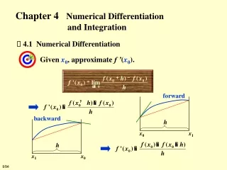
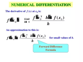
NUMERICAL DIFFERENTIATION The derivative of f(x) at x0 is: An approximation to this is: for small values of h. Forward Difference Formula
Find an approximate value for The exact value of
Assume that a function goes through three points: Lagrange Interpolating Polynomial
.............. (1) Alternate approach (Error estimate) Take Taylor series expansion of f(x+h) about x:
................. (2) .............. (1) 2 X Eqn. (1) – Eqn. (2)
The Second Three-point Formula Take Taylor series expansion of f(x+h) about x: Take Taylor series expansion of f(x-h) about x: Subtract one expression from another
Forward Difference Formula Error term Summary of Errors
First Three-point Formula Error term Summary of Errors continued
Second Three-point Formula Error term Summary of Errors continued
Example: Find the approximate value of with
Using the 2nd Three-point formula: The exact value of
The exact value of is 22.167168 Comparison of the results with h = 0.1
Second-order Derivative Add these two equations.
NUMERICAL INTEGRATION area under the curve f(x) between In many cases a mathematical expression for f(x) is unknown and in some cases even if f(x) is known its complex form makes it difficult to perform the integration.
Area of the trapezoid The length of the two parallel sides of the trapezoid are: f(a) and f(b) The height isb-a
Riemann Sum The area under the curve is subdivided into n subintervals. Each subinterval is treated as a rectangle. The area of all subintervals are added to determine the area under the curve. There are several variations of Riemann sum as applied to composite integration.
In Left Riemann sum, the left-side sample of the function is used as the height of the individual rectangle.
In Right Riemann sum, the right-side sample of the function is used as the height of the individual rectangle.
In the Midpoint Rule, the sample at the middle of the subinterval is used as the height of the individual rectangle.
Composite Trapezoidal Rule: Divide the interval into n subintervals and apply Trapezoidal Rule in each subinterval. where
Find by dividing the interval into 20 subintervals.
Composite Simpson’s Rule: Divide the interval into n subintervals and apply Simpson’s Rule on each consecutive pair of subinterval. Note that n must be even.
where Find by dividing the interval into 20 subintervals.