Scientific Computing Numerical Differentiation
Scientific Computing Numerical Differentiation. Dr. Guy Tel- Zur. Clouds. Picture by Peter Griffin, publicdomainpictures.net. Some Recent New Articles and Blog Posts. “ MY SLICE OF PIZZA ” Blog. ” - DIMACS Parallelism 2020: John Gustafson


Scientific Computing Numerical Differentiation
E N D
Presentation Transcript
Scientific ComputingNumerical Differentiation Dr. Guy Tel-Zur Clouds. Picture by Peter Griffin, publicdomainpictures.net
“MY SLICE OF PIZZA” Blog • ” - DIMACS Parallelism 2020: John Gustafson • “Throw out old Numerical Analysis textbooks! Algorithm designers have historically "measured" algorithm run times by counting the number of floating point operations / additions / multiplications. This made sense decades ago, when floating point arithmetic took 100 times as long as reading a word from memory. Now, one multiplication takes about 1.3 nanoseconds (to go through the entire pipeline; this underestimates throughput), compared to 50-100 nanoseconds for the memory access. Why do our algorithms measure the wrong thing? We should be counting memory accesses; it isn't reasonable to ignore the constant factor of 50.” • Slides are here
Computing in Science and Engineering • March/April 2011 – A few papers about Python! • Python for Scientists and Engineers • Python: An Ecosystem for Scientific Computing • Mayavi: 3D Visualization of Scientific Data • Cython: The Best of Both Worlds • The NumPy Array: A Structure for Efficient Numerical Computation
Code examples from “Python for Scientists and Engineers“ Another example (Guy): Demo: symbolicmath.py from sympy import exp f=lambda x: exp(-x**2) integrate(f(x),(x,-inf,inf)) See also: “From Equations to Code: Automated Scientific Computing” By Andy R. Terrel”, Computing in Science and Engineering, March-April 2011
Next Slides from Michael T. Heath – Scientific Computing • Source: http://www.cse.illinois.edu/heath/scicomp/notes/chap01.pdf
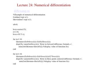
MHJ Chapter 3: Numerical Differentiation Should be f’c “2” stands for two points
Example code • 2nd derivative of exp(x) • Code in C++, we will learn more of the language features: • Pointers • Call by Value/Reference • Dynamic memory allocation • Files (I/O)
Call by value vs. call by reference • printf(“speed= %d\n”, v); // this is a call by value as the value of v won’t be changed by the function (printf) – which is desired • scanf(“%d\n”,&v); // this is a call by reference, we want to supply the address of v in order to set it’s value(s)
Analyzing an example code // This program module demonstrates memory allocation and data transfer // in between functions in C++ #include<stdio.h> #include<stdlib.h> int main(int argc, char *argv[]) { int a; // line 1 int *b; // line 2 a = 10; // line 3 b = new int[10]; // line 4 for(i = 0; i < 10; i++) { b[i] = i; // line 5 } func( a,b); // line 6 return 0; } // End: function main() void func( int x, int *y) // line 7 { x += 7; // line 8 *y += 10; // line 9 y[6] += 10; // line 10 return; // line 11 } // End: function func()
// // This program module // demonstrates memory allocation and data transfer in between functions in C++ #include<stdio.h> #include<stdlib.h> void func( int x, int *y); int main(int argc, char *argv[]) { int a; // line 1 int *b; // line 2 a = 10; // line 3 b = new int[10]; // line 4 for(int i = 0; i < 10; i++) { b[i] = i; // line 5 } func( a,b); // line 6 printf("a=%d\n",a); printf("b[0]=%d\n",b[0]); printf("b[1]=%d\n",b[1]); printf("b[2]=%d\n",b[2]); printf("b[3]=%d\n",b[3]); printf("b[4]=%d\n",b[4]); printf("b[5]=%d\n",b[5]); printf("b[6]=%d\n",b[6]); printf("b[7]=%d\n",b[7]); printf("b[8]=%d\n",b[8]); printf("b[9]=%d\n",b[9]); return 0; } // End: function main() void func( int x, int *y) // line 7 { x += 7; // line 8 *y += 10; // line 9 y[6] += 10; // line 10 return; // line 11 } // End: function func() תכנית משופרת Check program: demo1.cpp Under /lectures/02/code
Topics from MHJ Chapter 3 • Program 1: 2nd derivative of exp(x) in C++ • Program 2: Working with files • Program 3: Same as program #1 plus working with files • Program 4: The same in Fortran 90 • Error Estimation • Plotting the error using gnuplot
! • A reminder for myself: open DevC++ for the demos!) • I slightly modified “program1.cpp” from MHJ section 3.2.1 (2009 Fall edition): http://www.fys.uio.no/compphys/cp/programs/FYS3150/chapter03/cpp/program1.cpp • Install DevC++ on you personal laptop/computer and try it!
Explain program1.cpp Working directory: c:\Users\telzur\Documents\Weizmann\ScientificComputing\SC2011B\Lectures\02\code> Open DevC++ IDE for the demo Program description: // Program to compute the second derivative of exp(x). // Three calling functions are included // in this version. In one function we read in the data from screen, // the next function computes the second derivative // while the last function prints out data to screen. // The variable h is the step size. We also fix the total number // of divisions by 2 of h. The total number of steps is read from // screen Usage: > program1 <user input> 0.01 10 100 Examine the output: > type out.dat
program2.cpp • The book mentions program2.cpp which is in cpp and the URL is indeed a cpp code, but the listing below the URL is in C. • This demonstrates the I/O differences between C and C++
Working with files in C++ program2.cpp using namespace std; #include <iostream> int main(int argc, char *argv[]) { FILE *in_file, *out_file; if( argc < 3) { printf("The programs has the following structure :\n"); printf("write in the name of the input and output files \n"); exit(0); } in_file = fopen( argv[1], "r"); // returns pointer to the input file if( in_file == NULL ) { // NULL means that the file is missing printf("Can't find the input file %s\n", argv[1]); exit(0); } out_file = fopen( argv[2], "w"); // returns a pointer to the output file if( out_file == NULL ) { // can't find the file printf("Can't find the output file%s\n", argv[2]); exit(0); } fclose(in_file); fclose(out_file); return 0; }
program3.cpp • Usage: > program3 outfile_name • All the rest is like in program1.cpp
Now lets check the f90 version • Open in SciTEprogram1.f90 • In the image below: compilation and execution demo:
Content of exp(10)’’ computation • See MHJ section 3.2.2 and Fig. 3.2 (Fall 2009 Edition) • Text output with 4 columns: h, computed_derivative, log(h),ε >program1 Input: 0.1 10. 10 >more out.dat 1.00000E-001 2.72055E+000 -1.00000E+000 -3.07904E+000 5.00000E-002 2.71885E+000 -1.30103E+000 -3.68121E+000 2.50000E-002 2.71842E+000 -1.60206E+000 -4.28329E+000 1.25000E-002 2.71832E+000 -1.90309E+000 -4.88536E+000 6.25000E-003 2.71829E+000 -2.20412E+000 -5.48742E+000 3.12500E-003 2.71828E+000 -2.50515E+000 -6.08948E+000 1.56250E-003 2.71828E+000 -2.80618E+000 -6.69162E+000 7.81250E-004 2.71828E+000 -3.10721E+000 -7.29433E+000 3.90625E-004 2.71828E+000 -3.40824E+000 -7.89329E+000 1.95313E-004 2.71828E+000 -3.70927E+000 -8.44284E+000
Download and install Gnuplot http://www.gnuplot.info/
Visualization: Gnuplot • Reconstruct result from MHJ - Figure 3.2 using gnuplot • Gnuplot is included in Python(x,y) package! • Gnuplot tutorial: http://www.duke.edu/~hpgavin/gnuplot.html • Example: http://www.physics.ohio-state.edu/~ntg/780/handouts/gnuplot_quadeq_example.pdf • 3D Examples: http://www.physics.ohio-state.edu/~ntg/780/handouts/gnuplot_3d_example_v2.pdf
Can we explain this behavior? Computed for x=10
Error Analysis εro = Round-Off error The approximation error: Recall Eq. 3.4: The leading term in the error (j=1) is therefore:
The Round-Off Error (εro) • εro depends on the precision level of the chosen variables (single or double precision) Single precision If the terms are very close to each other, the difference is at the level of the round off error Double precision
hmin = 10-4 is therefore the step size that gives the minimal error in our case. If h>hmin the round-off error term will dominate
Summary • Next 3 slides are from: Michael T. Heath Scientific Computing • http://www.cse.illinois.edu/heath/scicomp/notes/chap08.pdf
Let’s upgrade our visualization skills! • Mayavi • Included in the Python(x,y) package • 2D/3D • User guide: http://code.enthought.com/projects/mayavi/docs/development/html/mayavi/index.html