Download
1 / 18
180 likes | 413 Vues
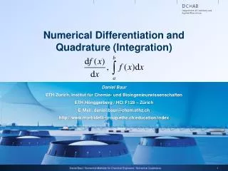
Numerical Differentiation and Quadrature (Integration ). Daniel Baur ETH Zurich, Institut für Chemie- und Bioingenieurwissenschaften ETH Hönggerberg / HCI F128 – Zürich E-Mail: daniel.baur@chem.ethz.ch http://www.morbidelli-group.ethz.ch/education/index . Numerical Differentiation.

E N D
Numerical Differentiation andQuadrature (Integration) Daniel BaurETH Zurich, Institut für Chemie- und BioingenieurwissenschaftenETH Hönggerberg / HCI F128 – ZürichE-Mail: daniel.baur@chem.ethz.chhttp://www.morbidelli-group.ethz.ch/education/index Daniel Baur / Numerical Methods for Chemical Engineers / Numerical Quadrature
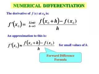
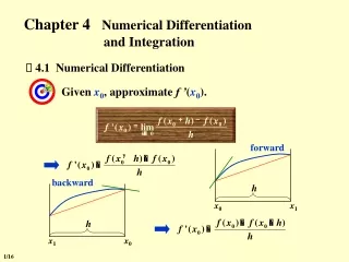
Numerical Differentiation • Problem:Though a derivative can be found for most functions, it is often impractical to calculate it analytically • Solution:Approximate the derivative numerically • First approach: • Remember that: • Therefore: for small h • Just how small should h be? Daniel Baur / Numerical Methods for Chemical Engineers / Numerical Quadrature
Example • Let us consider the following • h = 0.5, 0.05, 0.005 • For most applications,is a good starting point Daniel Baur / Numerical Methods for Chemical Engineers / Numerical Quadrature
Error as a Function of h Beware of the limits of numerical precision! Daniel Baur / Numerical Methods for Chemical Engineers / Numerical Quadrature
Better Alternatives • Instead of decreasing h, we could use better formulas • Symmetric midpoint formula: • Even more accurate, the five point formula: Daniel Baur / Numerical Methods for Chemical Engineers / Numerical Quadrature
Numerical Quadrature (Integration) • Problem:Generally, it is not possible to find the antiderivative (Stammfunktion) of a function f(x) in order to solve a definite integral in the interval [a,b] • Solution:Approximate the integral numerically • First approach:Divide the interval into n-1 sub-intervals and approximate the integral by the sum of the areas of the resulting rectangles Daniel Baur / Numerical Methods for Chemical Engineers / Numerical Quadrature
Rectangular Approximation b xn-1 a x1 x2 Daniel Baur / Numerical Methods for Chemical Engineers / Numerical Quadrature
Example • Let us consider a function where the antiderivative is easily found and integrate it in the interval a = 1, b = 10, h = 0.1: Matlab Integrator Daniel Baur / Numerical Methods for Chemical Engineers / Numerical Quadrature
Improvement • Use trapezoids instead of rectangles b xn-1 a x1 x2 Daniel Baur / Numerical Methods for Chemical Engineers / Numerical Quadrature
Cavalieri Simpson Rule • Further improve the result by using parabolas through each group of 3 points Parabola through f(a), f(x1), f(x2) b xn-1 a x1 x2 Daniel Baur / Numerical Methods for Chemical Engineers / Numerical Quadrature
Influence of h (or Number of Points) • How does the error change as a function of the number of points? Limit of numerical precision is reached Daniel Baur / Numerical Methods for Chemical Engineers / Numerical Quadrature
How does Matlab do it? • quad: Low accuracy, non-smooth integrands, uses adaptive recursive Simpson rule • quadl: High accuracy, smooth integrands, uses adaptive Gauss/Lobatto rule (degree of integration routine related to number of points) • quadgk: High accuracy, oscillatory integrands, can handle infinite intervals and singularities at the end points, uses Gauss/Konrod rule (re-uses lower degree results for higher degree approximations) • Degree p of an integration rule = Polynomials up to order p can be integrated accurately (assuming there is no numerical error) Daniel Baur / Numerical Methods for Chemical Engineers / Numerical Quadrature
Matlab Syntax Hints • All the integrators use the syntaxresult = quadl(@int_fun, a, b, ...); • int_funis a function handle to a function that takes one input x and returns the function value at x; it must be vectorized • Use parametrizing functions to pass more arguments to int_fun if neededf_new = @(x)int_fun(x, K); • f_new is now a function that takes only x as input and returns the value that int_fun would return when K is used as second input • Note that K must be defined in this command • This can be done directly in the integrator call:result = quadl(@(x)int_fun(x, K), a, b); Daniel Baur / Numerical Methods for Chemical Engineers / Numerical Quadrature
Exercise • Mass Transfer into Semi-Infinite Slab • Consider a liquid diffusing into a solid material • The liquid concentration at the interface is constant • The material block is considered to be infinitely long, the concentration at infinity is therefore constant and equal to the starting concentration inside the block c(z, t) c0 = const. c∞ = const. z 0 Daniel Baur / Numerical Methods for Chemical Engineers / Numerical Quadrature
Exercise (Continued) • Using a local mass balance, we can formulate an ODE • where j is the diffusive flux in [kg m-2 s-1] • With Δz 0, we arrive at a PDE in two variables jin jout z+Δz z Daniel Baur / Numerical Methods for Chemical Engineers / Numerical Quadrature
Exercise (Continued) • By combining this local mass balance with Fick’s law, a PDE in one variable is found: • The analytical solution of this equation (found by combination of variables) reads: Daniel Baur / Numerical Methods for Chemical Engineers / Numerical Quadrature
Assignment • Write a Matlab program to calculate and plot the concentration profile in the slab at different time points • Use the following values:c∞ = 0; c0 = 1; D = 10; t = 1, 10, 100Plot z from 1e-6 to 100 • I recommend using quadlfor the integration • Create a function of your own which calculates an integral with the trapezoidal method • Use the form: function F = trapInt(f, N, a, b) • Where f is a function handle to the function that is to be integrated,N is the number of points and a and b denote the interval • Use your function to solve the diffusion problem at t = 100 and compare it to the result you obtained with quadl Daniel Baur / Numerical Methods for Chemical Engineers / Numerical Quadrature
Assignment (Continued) • Improve your function by adding a convergence check: • In addition to computing the integral with Npoints, simultaneously do so with 2Npoints • If the two results differ by more than 10-6, double N and reiterate the calculation • This can be done either with a loop or with a recursive function • Terminate the calculation and issue a warning if N exceeds a certain amount • Extra: It is possible to implement the convergence check while still only calculating one integral per iteration (except in the first iteration). Can you do this? Daniel Baur / Numerical Methods for Chemical Engineers / Numerical Quadrature