Recombination Mapping
Recombination Mapping. Why . A fundamental problem in human genetics today is locating and identifying the specific gene responsible for a given genetic disease.

Recombination Mapping
E N D
Presentation Transcript
Why • A fundamental problem in human genetics today is locating and identifying the specific gene responsible for a given genetic disease. • However, the disease is just a phenotype, and gene responsible for that phenotype might be very different from what we would expect. • For instance, Lesch-Nyhan syndrome’s most spectacular manifestation is self-mutilating behavior. The Lesch-Nyhan gene codes for hypoxanthine-guanine phosphoribosyl transferase, which helps salvage nucleotides derived from the breakdown of nucleic acids. • So, we need to reduce the number of candidate genes to a manageable level. • Using the naturally occurring recombination process to map genes remains the best way to localize the gene responsible for a genetic disease. The goal is to reduce the amount of DNA that need to be searched to a small region, a few million base pairs or so. Below that level, molecular tools need to be employed.
Recombination Basics • in prophase of meiosis I, homologous chromosomes synapse (pair up) and crossing over occurs. The chromosomes break at approximately the same location and are rejoined to each other. • the recombinase enzyme complex catalyzes this reaction. • we examined the molecular details of this when we discussed gene conversion. A short region of DNA at the break point is a heteroduplex: composed of one DNA strand from each parent.
More Basics • Recombination appears in the offspring’s phenotype as exchange of marker genes on either side of the crossover. • Thus, to detect crossing over we examine two marker genes. The parent we are observing must be heterozygous for both genes. • if both dominant alleles are on one homologue and both recessives are on the other, the alleles are in coupling phase. • if one dominant and one recessive are on each homologue, the alleles are in repulsion. • coupling and repulsion are also use to describe relationships between co-dominant markers. • The marker alleles in an offspring are either in the Parental configuration (same as they were in the parents) or in the Recombinant configuration (marker exchange has occurred).
Map Distances • C-O occurs at random along chromosome--means that the closer 2 genes are, the less frequently recombination occurs. Basis for mapping. • Recombination Fraction (RF or theta or θ) is the percentage of recombinant gametes produced. • one complicating factor when looking at offspring: meiosis occurs in both parents. • RF is never more than 50%--due to only 2 of the 4 chromatids recombining • 1% recombination = 1 map unit = 1 centiMorgan (cM), but only for short distances. • for longer distances, double crossovers decrease observed recombination frequency. • two crossovers between marker genes leaves the markers in the parental configuration: no way to tell there were any crossovers. • Double crossovers should occur at frequency predictable from distances between genes, but there is also interference, which affects the chance for C-O in any interval. • interference: one crossover inhibits the occurrence of another nearby.
Mapping Function • We want a gene map to be calibrated in map units that accurately reflect the frequency of crossovers between genes. Thus we need to convert the observed recombination fraction into map units. • For a simple model of randomly placed crossovers and no interference, Haldane’s function works well: w = - ½ ln(1-2θ) , where w is map distance • this expression produces the curve on the previous slide • Interference complicates things, and a variety of functions can be used. Kosambi’s function is a common one: w = ¼ ln[(1+2θ) / (1-2θ)] • Interference has been estimated for human genes, and it seems to be a very small effect. For a 10 cM interval, only 0.01% of the potential crossovers is inhibited by interference. • Also, from a practical point of view, the main value of recombination mapping is finding a small region of DNA to search with molecular tools. Worrying about interference seems (to me) to be a lot of work for very little benefit. • Further, it is clear that a crossover is not equally probable at every nucleotide: at the level of the DNA sequence, recombination primarily occurs at hot spots with very little in between:
Chiasmata • Crossing over is visible in the microscope as chiasmata (which is the plural form of chiasma). • It is possible to count chiasmata. Each one counts as 50 map units (one crossover between 2 of the 4 DNA molecules at prophase of meiosis 1). • In male meiosis (testicular biopsy), one study shoed an average of 50.6 chiasmata per cell. Multiplying by 50, this gives 2530 cM as the length of the genetic map in males. • In female meiosis (between 16 and 24 weeks of fetal life), an average of 70.3 chiasmata per cell were seen. This gives a female map of 3515 cM. • Recombination mapping has given estimates of 2590 cM for males and 4281 for females. • So, females have more crossovers and a larger map than males. The total map length in humans is about 3000 cM.
Markers • What makes a good marker: • co-dominant (so homozygotes and heterozygotes can be distinguished) • many alleles at each locus (so most people will be heterozygous and different from each other) • many loci well distributed throughout the genome • easy to detect, especially with automated machinery • No system is perfect
Marker Systems • Originally, genetic markers were visible phenotypes and blood groups. There simply aren’t enough markers available, and many of them are dominant. Also, very few people display visible phenotypes that can be attributed to single genes. • before the advent of molecular markers, very few genes had been mapped, and most of them were on the X. • Protein electrophoresis. Isozymes are enzymes that have different electrophoretic mobility because they are produced by different alleles at the same gene. They are usually co-dominant, but frequently form dimers that can confuse interpretation. However, no more than 100 have ever been described, and many of these are not very polymorphic. Also, each enzyme requires a unique set of reaction conditions, which makes automation difficult.
More Marker Systems • Restriction Fragment length Polymorphisms (RFLPs). The original DNA-based marker system. These markers are (usually) single nucleotide polymorphisms which create or destroy a restriction site. Thus, they have only 2 alleles per locus. The original detection technique, Southern blots, were expensive, time-consuming and finicky (and radioactive too). • Microsatellites (SSRs). Lots of loci well scattered throughout the genome. Most loci have multiple alleles that are easily distinguishable. Detection is PCR-based, and there is some problem with DNA polymerase stuttering in PCR (which is also how new alleles are generated). The main problem is the need for gel electrophoresis to detect the alleles.
Single Nucleotide Polymorphisms • Single Nucleotide Polymorphisms (SNPs). The current method of choice. Each locus has a maximum of 4 alleles (with 2 being the usual case). But, there are very large numbers of SNP loci, often several per gene even within exons. And, detection can be done with assays that don’t require electrophoresis and so are very fast and easy to automate. • At present there are approximately 12 million human SNPs recorded in the NCBI database.
Fingerprinting Markers • Useful for forensics: distinguishing the DNA of one person from another. But not generally useful for mapping. • MHC locus. Lots of haplotypes, but all at one location of chromosome 6. • Minisatellites (Variable Number Tandem Repeats). Longer than microsatellites. Many alleles, but mostly clustered near telomeres. No general method of finding them. • Currently the FBI uses a set of 13 short tandem repeat markers for their forensic DNA work.
Mapping Techniques • Two point crosses: how far apart are two genes? This is done by the lod score method that we will discuss in detail shortly. • Three point crosses. Once a good genetic map is available, it is possible to map genes between pairs of other genes. This has the great advantage of being able to determine gene order, because one type of offspring can only occur by double crossovers, which are very rare compared to single crossovers. • Mapping of genes in sperm. There just aren’t enough people with a given mutant phenotype to map genes very closely. For DNA markers, one way around this is to map the genes in single sperm cells. There is a huge supply, and they are haploid, which eliminates the problem of linkage phase. The biggest problem here is that most interesting diseases don’t have phenotypes detectable in the DNA. • In general, linkage mapping suffers from the need to develop an accurate model of its inheritance: dominant (partial or complete), recessive. Incomplete penetrance is a big problem: people who have the mutant genotype but express the wild type phenotype. • But still, linkage mapping is the only way to locate the genes responsible for diseases whose cause is completely unknown.
LOD Score Mapping • The general problems with mapping genes in humans: small families, uncontrolled matings, uncertain paternity. • Thus you can’t set up a test cross, where one parent is a heterozygote and the other is homozygous for other alleles, and count parental and recombinant offspring. • Given a pedigree family, the lod score method involves determining the probability (the likelihood) of that family at different values of θ, the recombinant fraction. • Then, the method allows you to add probabilities across different families, even if some information about them is missing or ambiguous. Also, each family can start with different parental arrangements of markers, and can have different numbers and types of children. • The lod score method is an example of a maximum likelihood procedure. • The point of the maximum likelihood procedure is to estimate the value of a parameter that can’t be directly observed, in this case the recombination fraction. • The likelihood (probability) of an observed set of data (the phenotypes seen in a family, in this case) is calculated as a function of that parameter. • The parameter value that gives the maximum likelihood is taken as the best estimate of the parameter.
LOD Procedure • Start with a model of inheritance for the gene of interest, and work out an equation that gives the expected frequency of various types of offspring given an arbitrary value of θ. • Then, using a form of the binomial expansion, you determine the likelihood of your data (family) at a number of different values of θ. • Then, determine the odds (likelihood ratio): likelihood at each value of θ divided by the likelihood at θ = 0.5 (unlinked). • Then, take the base 10 logarithm of the odds ratio. This is the log of the odds, the lod score for each value of θ. • Add lod scores for all θ values between families. This is the beauty of logarithms: they can be added. Thus, data from many small families can be added to achieve a statistically significant value for θ.
Statistical significance • A lod score of 3.0 for some value of θ is considered the threshold for accepting that the two genes are linked, with a 5% chance of a false positive (p = 0.05). • A lod score of -2 is considered evidence for the genes not being linked. • Generally more than one value of θ will go over the 3.0 level. The θ with the highest lod score is the point estimate of the true map distance. All other adjacent θ values with a lod score of at least 1 less than the maximum value are considered the “support interval”, the region in which the true linkage value is found.
Calculating Expected Offspring Frequencies • Now for the real fun. • The point of recombination mapping is to determine the frequency of different kinds of gametes. This situation is most easily done in a test cross, where meiosis in only one parent needs to be considered. • We are now going to consider what happens when meiosis in both parents is relevant. • Three steps: • calculate gamete frequencies as a function of θ • calculate offspring genotype frequencies using a Punnett square • use a spreadsheet vary the value of θ and see what the resulting expected frequencies for the phenotypes are. • Consider a cross with 2 linked genes: • the disease gene has alleles R (dominant, normal) and r (recessive disease allele). • the marker gene is co-dominant, with alleles M1 and M2. • Assume we know the linkage phase in both parents: • the father is R M1 / r M2 • the mother is R M2 / r M1
Gamete Frequencies • So, for the father, • parental gametes: R M1 and r M2 • recombinant gametes: R M2 and r M1 • For the mother, • parental gametes: R M2 and r m1 • recombinant gametes: R M1 and r M2 • θ is the proportion of recombinant gametes. Since there are two recombinant gametes, each has a proportion of 1/2 θ. • 1- θ is the proportion of parental gametes. Each of the the two parental gametes has a proportion of ½(1- θ ). • So, for the father, R M1 and r M2 gametes have a proportion of ½(1- θ ) and R M2 and r M1 have 1/2 θ. • For the mother, R M2 and r M1 gametes have a proportion of ½(1- θ ) and R M1 and r M2 have 1/2 θ. • Put them on a Punnett Square
Combining Gametes • Now combine the gametes in each row and column. • Also multiply the gamete frequencies at each intersection of row and column. • Only 3 possibilities: • two parental gametes combining have a frequency of ¼ (1- θ)2 • two recombinant gametes combining have a frequency of ¼ θ2 . • a parental gamete and a recombinant gamete combining have a frequency of ¼ θ(1- θ).
Phenotype Frequencies • Recall that r is the recessive disease allele and R is dominant normal: thus RR and Rr give the same normal phenotype. (designated R_). rr gives the mutant disease phenotype. • M1 and M2 are co-dominant, so M1M1, M1M2, and M2M2 are all distinct phenotypes. • A total of 6 phenotypes divided among the 16 cells of the Punnett square. • Combine the equations for all cells that give the same phenotype, then do a little algebra to simplify things. • R_ M1M1 : ¼ (1- θ)2 + ¼ θ2 + ¼ θ(1- θ) = ¼ (θ2 - θ + 1) • R_ M1M2 : 4 * ¼ θ(1- θ) + ¼ (1- θ)2 + ¼ θ2 = ¼ (2θ - 2θ2 + 1) • R_ M2M2 : ¼ (1- θ)2 + ¼ θ2 + ¼ θ(1- θ) = ¼ (θ2 - θ + 1) • rr M1M1 : ¼ θ(1- θ) • rr M1M2 : ¼ (1- θ)2 + ¼ θ2 = ¼ (2θ2 -2θ + 1) • rr M2M2 : ¼ θ(1- θ)
Offspring Frequencies Varying with θ • Use the equations in a spreadsheet to calculate offspring frequencies for all recombination fractions from 0 (completely linked) to 0.5 (unlinked). • We now have the expected frequencies of all possible phenotypes at different values of θ.
Likelihood of a Family • Likelihood functions determine the probability of the observed data in terms of the parameter being estimated. • For lod scores, a version of the binomial expansion is used. • The binomial describes the probability of families with two different phenotypes • p = probability of a normal child • q = probability of a mutant child • n = total number of children • each term describes a different family composition • the exponents on p and q represent the number of children with each phenotype. • Consider a family of 3 children whose parents are heterozygous for a recessive genetic disease. • p = chance of normal child = ¾ • q = chance of mutant child = ¼ • Here, p3 is a family of 3 normal children, 3p2q is 2 normal plus 1 affected, 3pq2 is 1 normal plus 2 affected, and q3 is 3 affected. • Chance of 2 normal + 1 affected is described by the term 3p2q. Thus, 3 * (3/4)2 * 1/4 = 27/64.
Multinomial Distribution • Extending the binomial to more than two phenotypes is very simple: just add more components to each term. • For example, for 4 phenotypes, C p2q1r3s1 (where C is some coefficient) describes the probability of a family of 7 children, where 2 of them have the “p” phenotype, 1 has the “q” phenotype, 3 have the “r” phenotype, and 1 has the “s” phenotype. • The coefficients in front of each term represent the number of possible families of the given composition. For the binomial we can calculate the coefficients using Pascal’s triangle (or a useful formula). • However, for lod score mapping we don’t need to bother with the coefficients because they get divided out.
Likelihood Ratio • Using a spreadsheet, we first calculate the expected frequency of each type of offspring at different values of θ. • Then we use the data from actual families to calculate the likelihood of each family at each value of θ. • Then we take the likelihood ratio: divide the likelihood at each θ by the likelihood at θ = 0.50 (i.e. unlinked). • Then we take the logarithm (base 10) of each likelihood.
Example • Consider a family of 8 children: • R_ M1M1 : 2 children • R_ M1M2 : 2 children • R_ M2M2 : 2 children • rr M1M1 : 0 children • rr M1M2 : 1 child • rr M2M2 : 1 child • The expression we will use to determine likelihood is p1q3r2s1t1u0 where p, q, r, s, t, and u are the probabilities of the 6 types of offspring from a few slides back.
Results • The maximum for this example is at = 0.3. Of course, with a spread sheet it is easy to test more intermediate values. • Further analysis shows the maximum lod score is between 0.25 and 0.26, with a lod score of 0.354. • Clearly more families are needed to reach the significance level of 3.0
Some Complications • Sometimes the linkage phase is unknown. For example, the relevant parent has a genotype Dd M1M2, where D is a dominant disease allele. We don’t know whether D is in coupling with M1 or M2. • Linkage phase is usually determined by looking at the grandparents in a 3 generation family. If their phenotypes were Dd M1M3 and dd M2M4, we would know that D was linked to M1. • Dealing with this is easy in the lod score method: just calculate lod scores for both situations, where D M1 is parental and where D M2 is parental. Then, just add the likelihoods together and continue with the procedure, getting the likelihood ratio and the lod score. (This is an example of the OR rule of probability: the probability of either this happening or that happening is the sum of the two individual probabilities).