Download
1 / 67
680 likes | 772 Vues
Explore the construction, interpretation, and effect of confidence intervals on a population mean, including the use of t-procedures and critical points in statistical analysis. Understand how sample size impacts the accuracy of confidence intervals.

E N D
Chapter 8. Inferences on a Population Mean 8.1 Confidence Intervals 8.2 Hypothesis Testing 8.3 Summary
8.1 Confidence Intervals8.1.1 Confidence Interval Construction(1/8) • Confidence Intervals • A confidence interval for an unknown parameter θis an interval that contains a set of plausible values of the parameter. • It is associated with a confidence level1-, which measures the probability that the confidence interval actually contains the unknown parameter value. • Confidence levels of 90%, 95%, and 99% are typically used.
8.1.1 Confidence Interval Construction(2/8) • Inferences on a Population Mean • Inference methods on a population mean based upon the t-procedure are appropriate for large sample sizes n ≥ 30 and also for small sample sizes as long as the data can reasonably be taken to be approximately normally distributed. • Nonparametric techniques (Chapter 15) can be employed for small sample sizes with data that are clearly not normally distributed.
8.1.1 Confidence Interval Construction(3/8) • Two-Sided t-Interval • A confidence interval with confidence level 1- for a population mean based upon a sample of n continuous data observations with a sample mean and a sample standard deviation s is • The interval is known as a two-sided t-interval or variance unknown confidence interval.
8.1.1 Confidence Interval Construction(4/8) • A two-sided t-interval
8.1.1 Confidence Interval Construction(5/8) • The length of two-sided t-interval is • As the standard error of decreases, so that becomes a more “accurate” estimate of . • The length of a confidence interval also depends upon the confidence level. As the confidence level increases, the length of the confidence interval also increase.
8.1.1 Confidence Interval Construction(6/8) • We know that and so the definition of the critical point of the t-distribution ensures that
8.1.1 Confidence Interval Construction(7/8) • And • This probability statement should be interpreted as saying that there is a probability of 1- that the random confidence interval limits take values that “straddle” the fixed value .
8.1.1 Confidence Interval Construction(8/8) • Technically speaking, has a t-distribution only when the random variables are normally distributed. • Nevertheless, the central limit theorem ensures that the distribution of is approximately normal for reasonably large sample sizes, and in such cases it is sensible to construct t-intervals regardless of the actual distribution of the data observations.
Sample size n = 60 Confidence level 90%: t0.05,59 = 1.671 Confidence level 95%: t0.025,59 = 2.001 Confidence level 99%: t0.005,59 = 2.662 Example 14 : Metal Cylinder Production (p.365) • Data : 60 metal cylinder diameters (page 290, Figure 6.5). • Summary statistics: n = 60 Median = 50.01 Max. = 50.36 = 49.999 Upper quartile = 50.07 Min. = 49.74 s = 0.134 Lower quartile = 49.91 • Critical points:
Example 14 : Metal Cylinder Production(2/4) • Confidence interval with confidence level 90%: • Confidence interval with confidence level 95%: • Confidence interval with confidence level 99%:
49.970 50.028 =49.999 90% 49.964 50.033 =49.999 95% 49.953 50.045 =49.999 99% Example 14 : Metal Cylinder Production(3/4) • Confidence intervals for mean metal cylinder diameter
Example 14 : Metal Cylinder Production(4/4) • Conclusion with confidence interval: With over 99% certainty, the average cylinder diameter lies within 0.05 mm of 50.00mm, that is, within the interval (49.95, 50.05). • Comment: It is important to remember that this confidence interval is for the mean cylinder diameter, and not for the actual diameter of a randomly selected cylinder.
8.1.2 Effect of the Sample Size on Confidence Intervals(1/4) • Recall: • For a fixed critical point, a confidence interval length L is inversely proportional to the square root of the sample size n. • Notice that this dependence of the critical point on the sample size also serves to produce smaller confidence intervals with large sample sizes.
8.1.2 Effect of the Sample Size on Confidence Intervals(2/4) • If a confidence interval with a length no large than L0 is required, then sample size must be used. This inequality can be used to find a suitable sample size n if approximate values or upper bounds are used for t/2, n-1 and s.
8.1.2 Effect of the Sample Size on Confidence Intervals(3/4) • Example (p. 364): For the mean thickness of plastic sheets, an experimenter wishes to construct a 95% confidence interval with a length no larger than L0 = 2.0 mm. • Known fact: the standard deviation (s) 4.0 mm • Assumption: t0.025, n-1 2.1, for a large enough sample size • Then a sample size is
8.1.2 Effect of the Sample Size on Confidence Intervals(4/4) • Additional sampling: • For a sample size n1 and a sample standard deviation s, the length of the confidence interval is • To reduce the confidence interval length to L0 < L, the size of the additional sample required is
Example 14 : Metal Cylinder Production (p. 365) • n = 60, 99% confidence interval (49.953, 50.045) and confidence length = 0.092 mm • Question: How much additional sampling is required to provide the increased precision of a confidence interval with a length of 0.08 mm at the same confidence level? • Answer: A total sample size required is • Therefore, an additional sample of at least 80-60 = 20 cylinders is needed.
8.1.4 Simulation Experiment(1/2) • Figure 8.8(page 369) shows the 500 simulation results (a mean of = 10, a sample size of n = 30) and 95% confidence intervals. • Notice that, in simulations 24 and 37, the confidence intervals do not include the correct value = 10. • Each simulation provides a 95% confidence interval which has a probability of 0.05 of not containing the value = 10.
8.1.4 Simulation Experiment(2/2) • Since the simulations are independent of each other, the number of simulations out of 500 for which the confidence interval does not contain = 10 has a binomial distribution with n = 500 and p = 0.05. • In practice, an experimenter observes just one data set, and it has a probability of 0.95 of providing a 95% confidence interval that does indeed straddle the true value .
8.1.5 One-Sided Confidence Intervals(1/4) • One-Sided t-Interval: One-sided confidence intervals with confidence levels 1- for a population mean based on a sample of n continuous data observations with a sample mean and a sample standard deviation s are which provides an upper bound on the population mean , and which provides a lower bound on the population mean .
8.1.5 One-Sided Confidence Intervals(2/4) • c.f. Since the definition of the critical point t,n-1 implies that
8.1.5 One-Sided Confidence Intervals(3/4) This may be rewritten so that is a one-sided confidence interval for with a confidence level of 1-.
One-sided(upper bound) Two-sided One-sided(lower bound) 8.1.5 One-Sided Confidence Intervals(4/4) • Figure 8.10: Comparison of two-sided and one-sided confidence intervals
Example 45 : Hospital Worker Radiation Exposures • n = 28, sample mean = 5.145, • sample standard deviation s = 0.7524, • critical point t0.01, 27 = 2.473. • 99% one-sided confidence interval for is • Consequently, with a confidence level of 0.99 the experimenter can conclude that the average radiation level at a 50cm distance from a patient is no more than about 5.5.
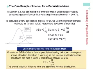
8.1.6 z-Intervals(1/2) • Two-Sided z-Interval If an experimenter wishes to construct a confidence interval for a population mean based on a sample of size n with a sample mean and using an assumed known value for the population standard deviation , then the appropriate confidence interval is which is known as a two-sided z-interval or variance known confidence interval.
8.1.6 z-Intervals(2/2) • One-Sided z-Interval One-sided 1- level confidence intervals for a population mean based on a sample of n observations with a sample mean and using a known value of the population standard deviation are These confidence intervals are known as one-sided z-intervals. and
8.2 Hypothesis Testing8.2.1 Hypotheses(1/2) • Hypothesis Tests of a Population Mean • A null hypothesisH0 for a population mean is a statement that designates possible values for the population mean. • It is associated with an alternative hypothesisHA, which is the “opposite” of the null hypothesis. • A two-sided set of hypotheses is H0 : = 0 versus HA : ≠ 0 for specified value of .
8.2.1 Hypotheses(2/2) • A one-sided set of hypotheses is either H0 : 0 versus HA : >0 or H0 : ≥ 0versusHA : <0
Example 14 : Metal Cylinder Production • The machine that produces metal cylinders is set to make cylinders with a diameter of 50 mm. • The two-sided hypotheses of interest are H0 : = 50 versus HA : ≠ 50 where the null hypothesis states that the machine is calibrated correctly.
Example 47 : Car Fuel Efficiency • A manufacturer claim : its cars achieve an average of at least 35 miles per gallon in highway driving. • The one-sided hypotheses of interest are H0 : ≥ 35 versusHA : < 35 • The null hypothesis states that the manufacturer’s claim regarding the fuel efficiency of its cars is correct.
8.2.2 Interpretation of p-values(1/4) • Types of error • Type I error: An error committed by rejecting the null hypothesis when it is true. • Type II error: An error committed by accepting the null hypothesis when it is false. • Significance level • is specified as the upper bound of the probability of type I error.
8.2.2 Interpretation of p-values(2/4) • p-value of a test (or observed level of significance) • Definition: The p-value of a test is the probability of obtaining a given data set or worse when the null hypothesis is true. • A data set can be used to measure the plausibility of null hypothesis H0 through the construction of a p-value. • The smaller the p-value, the less plausible is the null hypothesis. (why?)
8.2.2 Interpretation of p-values(3/4) • Rejection of the Null Hypothesis • If a p-value is smaller than the significance level, then the hypothesis H0 is rejected in favor of the alternative hypothesis HA. • Acceptance of the Null Hypothesis • A p-value larger than 0.10 is generally taken to indicate that the null hypothesis H0 is a plausible statement. The null hypothesis H0 is therefore accepted. • However, this does not mean that the null hypothesis H0 has been proven to be true.
8.2.2 Interpretation of p-values(4/4) • Intermediate p-values • A p-value in the range 1% ~ 10% is generally taken to indicate that the data analysis is inconclusive. There is some evidence that the null hypothesis is not plausible, but the evidence is not overwhelming.
Example 14 : Metal Cylinder Production • Q : whether the machine can be shown to be calibrated incorrectly. • H0 : = 50, HA : ≠ 50 • With a small p-value, • The null hypothesis is rejected and the machine is demonstrated to be miscalibrated. • With a large p-value, • The null hypothesis is accepted and the experimenter concludes that there is no evidence that the machine is calibrated incorrectly.
8.2.3 Calculation of p-values • Two-sided t-test • Consider testing
One-sided t-test • Consider testing • Then • Consider testing • Then
Example 14 : Metal Cylinder Production H0: = 0 versus HA: ≠ 0 • The data set of metal cylinder diameters: n = 60, = 49.99856, s = 0.1334 • 0 = 50.0 • p-value = 2 xP(X≥0.0836),X ~ t-distribution with n-1=59 d.f. • p-value = 2 x 0.467 = 0.934 • With such a large p-value, the null hypothesis is accepted. t59 distribution 0.467 0 ltl=0.0836
Example 47 : Car Fuel Efficiency (1/2) • n=20, • the fuel efficiency with a sample mean =34.271 miles/gallon • sample standard deviation s=2.915 miles/gallon. • 0 = 35.0 • The alternative hypothesis is HA: < 35, so that where X has a t-distribution with n-1=19 d.f.
Example 47 : Car Fuel Efficiency (2/2) • The value can be shown to be p-value = 0.1386. • This p-value is larger than 0.10 and so the null hypothesis should be accepted. t19 distribution -1.119 0 p-value
8.2.4 Significance Levels(1/14) • Significance Level of a Hypothesis Test • A hypothesis test with a significance level or size rejects the null hypothesis H0 if a p-value smaller than is obtained and accepts the null hypothesis H0 if a p-value larger than is obtained. • P-values are more informative than knowing whether a size test accepts or rejects the null hypothesis. (Why?)
8.2.4 Significance Levels(2/14) • Two-Sided Problems • Two-Sided Hypothesis Test for a Population Mean • A size test for the two-sided hypotheses rejects the null hypothesis H0 if the test statistic ltl falls in the rejection region and accepts the null hypothesis H0 if the test statistic ltl falls in the acceptance region • What is the role of here? H0: = 0 versus HA: ≠ 0
Example 14 : Metal Cylinder Production H0: = 0 versus HA: ≠ 0 • The data set of metal cylinder diameters gives a test statistic of ltl = 0.0836 • =0.10 t0.05,59=1.671 • =0.05 t0.025,59=2.001 • =0.01 t0.005,59=2.662 • The test statistic is smaller than each of these critical points, and so the hypothesis tests all accept the null hypothesis. • The p-value is therefore known to be larger than 0.10, and in fact the previous analysis found the p-value to be 0.934.
8.2.4 Significance Levels(3/14) • Relationship Between Confidence Intervals and Hypothesis Tests • The value 0 is contained within a 1- level two-sided confidence interval if the p-value for the two-sided hypothesis test H0: = 0 versus HA: ≠ 0 is larger than .
8.2.4 Significance Levels(4/14) • If 0 is contained within the 1- level confidence interval, the hypothesis test with size accepts the null hypothesis, and • if 0 is not contained within the 1- level confidence interval, the hypothesis test with size rejects the null hypothesis.
8.2.4 Significance Levels(5/14) • (FIGURE 8.36, Page 399)
Example 14 : Metal Cylinder Production (1/2) • A 90% two-sided t-interval for the mean cylinder diameter was found to be (49.970, 50.028). • This contains the value 0=50.0 and so is consistent with • the hypothesis testing problem H0: = 50.0 versus HA: ≠ 50.0 having a p-value of 0.934, so that the null hypothesis is accepted at size =0.10.
Example 14 : Metal Cylinder Production (2/2) • The 90% confidence interval implies that the hypothesis testing problem H0: = 0 versus HA: ≠ 0 has a p-value larger than 0.10 for 49.970050.028 and a p-value smaller than 0.10 otherwise. (Why ?)
8.2.4 Significance Levels(6/14) • One-Sided Inferences on a Population Mean(H0: 0) (p.401) • A size test for the one-sided hypothesis H0: 0 versus HA: > 0 rejects the null hypothesis when t > t,n-1 and accepts the null hypothesis when t t,n-1