Download
1 / 30
300 likes | 503 Vues
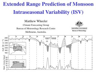
Extended Range Prediction of Monsoon Intraseasonal Variability (ISV). Matthew Wheeler Climate Forecasting Group Bureau of Meteorology Research Centre Melbourne, Australia. Acknowledgements.

E N D
Extended Range Prediction of Monsoon Intraseasonal Variability (ISV) Matthew Wheeler Climate Forecasting Group Bureau of Meteorology Research Centre Melbourne, Australia.
Acknowledgements Harry Hendon, Duane Waliser, Klaus Weickmann, Xianan Jiang, Harun Rashid, and Nicholas Savage contributed to this presentation. And I thank the local organising committee for this invitation.
Introduction Recent research has started to fill the gap that has traditionally existed between weather (~days) and climate (~seasons) prediction. E.g. Waliser et al. (1999), Lo and Hendon (2000), Wheeler and Weickmann (2001), Goswami and Xavier (2003), Webster and Hoyos (2004), and review by Waliser (2005). Due to the difficulties in accurately representing ISV in dynamical models, however, most of this research and development has been with empirical schemes. Also, due to the prominence of the MJO on this time scale, it is the MJO that has received most attention, especially, but not exclusively, in austral summer.
Here, I thus also concentrate on the MJO. In particular, I will: • Discuss two approaches to empirical prediction at BMRC, • Suggest a statistical benchmark for MJO prediction, and • Examine a MJO diagnostic for dynamical forecast models. • The work presented draws upon, and provides input to, two international working groups: • The Experimental MJO Prediction Projecthttp://www.cdc.noaa.gov/MJO/ • U.S. CLIVAR MJO Working Grouphttp://www.usclivar.org/Organization/MJO_WG.html
Two approaches to empirical prediction at BMRC a) Wavenumber-frequency filtering (very briefly) http://www.bom.gov.au/bmrc/clfor/cfstaff/matw/maproom/OLR_modes/ (operating for 7 years) b) Projection of daily observations onto combined EOFs of OLR, u850, and u200 to get two indices - what we call “Real-time Multivariate MJO” (RMM) 1 and RMM2. http://www.bom.gov.au/bmrc/clfor/cfstaff/matw/maproom/RMM/ (operating for 4 years)
1/ Monitoring and forecast from 16th January a) Wavenumber-frequency filtering of OLR 2/ Monitoring and forecast from 5th February (20 days later) 16th Jan As described by Wheeler and Weickmann (MWR, 2001)
Are these MJO prediction relevant to the monsoons? Correlation skill in Southern Summer for Day 15 Correlation skill in Northern Summer for Day 15
b) The Real-time Multivariate MJO (RMM) Index Index described by Wheeler and Hendon (2004). Statistical forecasts with index described by Maharaj and Wheeler (2005) and Jiang et al. (2007). The idea is that by projecting daily observed data (with long-time scale components carefully removed) onto the MJO’s multivariate spatial structure, you can isolate the signal of the MJO without the need for a band-pass time filter. EOFs of the combined fields of 15°S to 15°N-averaged OLR, u850, and u200, for all seasons.
Madden and Julian (1972) The pair of EOFs describe the convectively-coupled vertically-oriented circulation cells of the canonical MJO, as is detectable in all seasons.
It is thus convenient to view the state of the MJO in the two-dimensional phase space defined by the two EOFs. For example, looking at the 40 days up to 17th July 2007. We can use this index for empirical prediction.
Can form season-specific MJO composites using the seasonally-independent index. JJA RMM phase space for all days in JJA from 1974 to 2006. Approximately 200 days in each phase DJF RMM phase space for all days in DJF from 1974 to 2006.
MJO composite for JJA Reproduces some (~1/2) of the northward propagation in the Indian monsoon.
MJO composite for DJF Reproduces the southward excursion of convection into northern Australia.
Example MJO impact on rainfall (DJF) Probability that the weekly rainfall accumulation will exceed the upper tercile.
Can forecast RMM1 and RMM2 values using multiple linear regression RMM1(lag)=a1+b1RMM1(0) +c1RMM2(0) RMM2(lag)=a2+b2RMM1(0) +c2RMM2(0) where a1,a2,b1,b2,c1, and c2 are computed independently for each lag, and are a smoothly varying function of the time of year. Example from 17th July 15 day forecast (for 1st August) Skill as measured by the correlation coefficient 0.5 for a 15-day forecast (Maharaj and Wheeler 2005)
Similarly, can forecast any field using seasonally-varying, lagged, multiple linear regression against RMM1,RMM2 at Day 0. OLR and 850hPa wind anoms Initial Condition on 17 July, 2007 15-day forecast for 1st August
Skill of RMM-based predictions: Correlations of the predicted OLR anomalies with observed OLR (100-day high-pass) 15-day forecasts Southern Summer 15-day forecasts Northern Summer Only modest skill (like other empirical schemes), but a useful benchmark for dynamical MJO forecasts… (Jiang et al. 2007)
MJO forecast skill as a function of MJO phase: Is there a statistical MJO predictability barrier? Less skill for forecasts going through Phase 2. But drop in skill is only relatively minor. Figure courtesy of Xianan Jiang
A MJO diagnostic for dynamical forecast models A current activity of the US-CLIVAR MJO Working Group (Waliser/Sperber) (http://www.usclivar.org/Organization/MJO_WG.html) Project numerical model forecast data onto the same two RMM EOFs that were derived from observations. EOFs of the combined fields of 15°S to 15°N-averaged OLR, u850, and u200
Projection of daily analyses/model forecasts onto EOFs provides a diagnostic with which to measure the state of the MJO in both observations and model forecasts. Two examples: Obs + empirical forecast Obs + dynamical forecast #1 1st August 1st August Met Office Global and Regional Ensemble Prediction System Daily-updated dynamical forecasts available from http://www.cdc.noaa.gov/MJO/Forecasts/index_phase.html
Projection of daily analyses/model forecasts onto EOFs provides a diagnostic with which to measure the state of the MJO in both observations and model forecasts. Two examples: Obs + empirical forecast Obs + dynamical forecast #2 1st August 1st August 1st August NCEP Global Ensemble Prediction System
Latest ten forecasts from the Bureau of Meteorology’s coupled model (POAMA). Initial conditions for each forecast are 1 day apart (as labelled, starting on 9th July). Coloured lines show the trajectories of 30-day forecasts, with a black dot placed every 5 days. Ensemble mean (blue curve) is mean of just the last 5 forecasts. 15th August 1st August
What have the observations done up until yesterday? In this case, the dynamical models appeared to have performed reasonably well, as the observations have reproduced the relatively slow eastward propagation.
But how skilful are these dynamical forecasts in a general sense? Our benchmark statistical forecast is provided by lagged linear regression with RMM1 and RMM2 as predictors. Correlation skill of this benchmark is ~0.5 for a 15-day forecast (Maharaj and Wheeler 2005) For POAMA we have a comprehensive hindcast dataset with which to assess its skill (10-member ensemble started on the 1st of each month during 1980-2005).
POAMA example hindcasts and observations. When assessed using all seasons, correlation skill ~0.45 at 15 days! A little less than our statistical benchmark, despite POAMA having a better than average MJO.
For predictions of the total anomaly field (i.e., not just the MJO component), dynamical models look a little better. Experimental MJO Prediction Program (http://www.cdc.noaa.gov/MJO/) NCEP ENS = Ensemble mean of 2004 version of the GFS operational model (T254 L64). CDC ENS = Ensemble mean of forecasts from frozen version of MRF model corrected for model systematic errors (“Reforecast Project”). Image courtesy of Klaus Weickmann. See Waliser et al. (BAMS, 2006)
Summary • Most work on intraseasonal prediction has concentrated on the MJO, for good reason! • Empirical MJO prediction schemes, of various sorts, provide skill in the region of the Asian-Australian monsoon out to about 20 days. • For a benchmark statistical prediction, we suggest use of the Real-time Multivariate MJO (RMM) indices, and lagged linear regression. • RMM phases/phase space are also very useful for impact studies (e.g. impact on rainfall), and for diagnosing the state of the MJO in dynamical model forecasts. • Through our increased focus on the MJO, as allowed by these simple diagnostics, further improvements in the dynamical models will hopefully result (but that requires our full encouragement of model developers!).