Download
1 / 33
330 likes | 471 Vues
Summary of results on sample GX140. Data and Macrospin simulation. System. Ta(5 nm)/Cu(30 nm)/Pt(3nm) [Co(0.25nm) /Pt(0.52nm)]*4/ Co(0.25nm)/[Ni(0.6 nm)/Co (0.1 nm)]*2 /Cu(4nm )/ [Co (0.1 nm) /Ni(0.6 nm)]*2/Co(0.2 nm) / Pt(3 nm)/ Cu(20 nm)/ Ta(5 nm). Free Layer. Reference Layer. Easy Axis.

E N D
Summary of results on sample GX140 Data and Macrospin simulation
System Ta(5 nm)/Cu(30 nm)/Pt(3nm)[Co(0.25nm) /Pt(0.52nm)]*4/ Co(0.25nm)/[Ni(0.6 nm)/Co (0.1 nm)]*2/Cu(4nm)/[Co (0.1 nm) /Ni(0.6 nm)]*2/Co(0.2 nm)/Pt(3 nm)/ Cu(20 nm)/ Ta(5 nm) Free Layer Reference Layer Easy Axis
Phase diagram of 100x100nm sampleField Along easy axis I=0.003+0.033B P AP I=-0.007-0.0375B We have a coercive field of ~0.1T
Phase diagram of 100x100nm sampleField AT 45DEGREES I=0.003+0.032B P AP I=-0.007- 0.023B We have a coercive field very close to the on axis case
Pulse diagram fitting of 100x100nm sampleField Along Easy AxisP->AP
Pulse diagram fitting of 100x100nm sampleField at 30degreesAP->P
Pulse diagram of 100x100nm sampleField at 45degreesp->AP Low resolution measurements
Pulse diagram fitting of 100x100nm sampleField at 45 degreesP->AP
Pulse diagram fitting of 50x50nm sampleField along easy axisAP->P
Extrapolated Critical Currents Field along easy axis 100x100nm
Extrapolated Critical Currents Field along easy axis 50x50nm
Extrapolated Critical Currents Field at 30 degrees
Extrapolated Critical Currents Field at 45degrees
Macrospintheory • J.Z Sun, PRB62, Spin current interaction with a monodomain magnetic body A [Hz/V] characterizes dynamic evolution
Macrospin simulation parameters100x100nm sample • Coercive field (Bc): hysteresis curve0.1T • Dipolar field(Hdip): asymmetry of hysteresis curve0.02T (not included in simulation) • Saturation Magnetization (Ms): average of Co and Ni saturation magnetization weighted by thickness713000 A/m • Anisotropy constant(K): deduced from the coercive field and Ms3.55e5 J/m3
Macrospin simulation parameters • ~1.17 deduced from extrapolated critical currents • Polarization(P~0.2): extracted from fitting parameter A • Damping constant : deduced from previous values~0.23 Asymmetry of spin torque, deduced from phase diagram Current/Amplitude conversion factor
Phase Diagram P P AP AP
Extrapolated Critical Amplitude SimulationAP->P