Cost-volume-profit analysis
CHAPTER 9. Cost-volume-profit analysis. 9.1. Curvilinear cost-volume graph. 1. Results in two break-even points. 2. Note the shape of the total cost function: • initial steep rise, levels off, followed by a further steep rise.

Cost-volume-profit analysis
E N D
Presentation Transcript
CHAPTER 9 Cost-volume-profit analysis
9.1 Curvilinear cost-volume graph 1. Results in two break-even points. 2. Note the shape of the total cost function: • initial steep rise, levels off, followed by a further steep rise. 3. The total revenue line initially rises steeply, then levels off and declines.
9.2 Linear CVP relationships
9.3 • Linear cost–volume–profit model • Constant variable cost and selling price is assumed. • Only one break-even point, and profit increases as volume increases. • The diagram is not intended to provide an accurate representation for all levels of output. The objective is to provide an accurate representation of cost and revenue behaviour only within the relevant range of output.
9.4 • Fixed cost function • Within the short term the firm anticipates that it will • operate between output levels Q1 and Q2 and commits itself to fixed costs of 0X. • Costs are fixed in the short term, but can be changed in the longer term.
9.5a • CVP analysis: non-graphical computations • 1. Example 1 • Fixed costs per annum £60 000 • Unit selling price £20 • Unit variable cost £10 • Relevant range 4 000 - 12 000 units • 2. Break-even point • Fixed costs = £60 000/£10 = 6 000 units Contribution per unit • 3. Units to be sold to obtain a £30 000 profit: • Fixed costs + desired profit = £90 000/£10 = 9 000 units • Contribution per unit
9.5b • 4. If unit fixed costs and revenues are not given, the break-even point (expressed in sales values) can be calculated as follows: • Total fixed costs x Total sales = £120 000 • Total contribution • 5. Profit volume ratio = Contribution x 100 = 50% • Sales revenue • 6. Percentage margin of safety = • Expected sales - Break-even sales = 25% for £160 000 sales • Expected sales
9.6 Break-even chart for Example 1
9.7 Contribution chart for Example 1
9.8 Profit-volume graph for Example 1
9.9a CVP analysis assumptions 1. All other variables remain constant • e.g.sales mix, production efficiency, price levels, production methods. 2. A single product or constant sales mix 3. Total costs and total revenues are linear functions of output 4. The analysis applies only to the relevant range. 5. The analysis applies only to a short-term horizon.
9.9b Example Product X Product Y Unit contribution £12 £8 Budgeted sales mix 50% 50% Actual sales mix 25% 75% Fixed costs are £180 000 Budgeted BEP = £180 000 /£10 (a) = £18 000 units Actual BEP = £180 000 /£9 (b) = 20 000 units (a) (50% × £12) + (50% × £8) (b) (25% × £12) + (75% × £8)