- "Understanding Resistivity Survey Method in Geological Exploration" -
Learn about resistivity survey method and factors affecting ground resistivity. Discover the field set-up, drawbacks, and assets of this technique in subsurface analysis. -

- "Understanding Resistivity Survey Method in Geological Exploration" -
E N D
Presentation Transcript
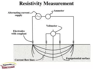
Resistivity Method One of the main distinctions between the terrain conductivity and resistivity methods is that the resistivity method employs direct injection of current into the ground whereas the terrain conductivity method operates through the use of induced current flow. In the picture above you can see that in the resistivity survey current electrodes are driven into the ground at intervals along a profile. Ground resistivity is then measured directly as a potential difference between potential electrodes.
What factors affect resistivity? 1. Porosity: shape and size of pores, number 2. Permeability: size and shape of interconnecting passages 3. The extent to which pores are filled by water, i.e. the
Temporal Change From Mike Solt, 2002
Conductivity reduction over 2 year period From Mike Solt, 2002
Field Set-up (schematic) Our task is not to determine electric force, electric field intensity or charge associated with an unknown object. Generally we are dealing with an ionized solution and the charge balances out. The net charge is zero. To characterize the conductor we have to upset the balance - create differences in the electrical potential throughout the conductor and observe the effect - make current flow. We want to determine the resistivities of various layers or zones. That is the basic information that we interpret and model
DRAWBACKS Direct current injection is required. Can be difficult to get current into the ground so that little or no current reaches the zone of interest and hence its resistivity has little effect on the apparent resistivity measured by the resistivity meter. Labor intensive and time consuming- ASSETS The resistivity method is generally more versatile than the terrain conductivity survey. There are fewer restrictions on electrode spacing The ability to employ a great number of electrode spacings in a sounding, for example, provides a much more comprehensive data base of measurements from which to infer the distribution of subsurface resistivity variation.
By convention the direction of current flow is considered to be the direction in which positive charges move. Hence if you are following the progress of an electron in a wire, current flow is opposite the direction of the electron movement.
+ - We also associate certain vector orientations with positive and negative charges. The force or electric field intensity arrows emerge from the positive charges. Thus as you might have guessed our reference charge is positive (likes repel). Conversely, by convention, the field lines associated with a negative charge point toward it.
+ - + - Source Sink Direction of positive charge flow Sink Source
Current i = current q = charge t = time Cross sectional area A Charge q Drift Velocity v A chargewill move through a conductor at some average or root-mean-square velocty
The quantitative aspects of resistivity methods that we will deal with all stem directly from Ohm’s law. Because resistance is so dependant upon the geometry of the conductor, we deal with resistivity rather than resistance. The form of Ohm’s law we will use is where is the resistivity.
- + d1 A Next let’s consider how apparent ground resistivity is measured given the typical setup of current and potential electrodes. To do this we have to compute the potential difference between the terminals of the voltmeter. But first consider the following diagram and ask what is the potential at point A? d2
- + d1 A Recall that the potential - i.e. Ohm’s law. Consider first, what is the potential at A due to the positive current electrode located a distance d1 away? Medium with resistivity In this diagram l is d1. What is A?
- + d1 A A will be the area over which the current i spreads out through the subsurface. That area will be the area of a hemisphere with radius d1 or just 2d12. Thus -
Obviously the potential at point A will be the sum of two potentials - one with respect to the positive electrode, V+ and the other with respect to the negative electrode, V- . By a similar line of reasoning - Note that we include the negative sign associated with the negative charge of the sink electrode.
Hence, the potential at point A associated with the contributions from both the positive and negative electrodes will be the sum of these two potentials, or just or just
- + A B V d1 d2 d3 d4 Through a similar line of reasoning - the potential difference measured by the voltmeter between potential electrodes located at points A and B on the surface will be VA - VB.
- + M N V d1 d2 d3 d4 A B
Given that The potential difference
This equation is easily solved for the resistivity The term Is referred to as a geometrical factor and the apparent resistivity a is often written as
Where G is We can see that the geometrical factor contains information about the positioning of the current and potential electrodes in the survey - and as you have probably guessed there are several ways to arrange the potential and current electrodes.
One of the most commonly used electrode configurations is known as the Wenner array. In this setup a constant spacing is maintained between the electrodes in the array. That spacing is usually referred to as a. - + V d1=a a d4=a d2=2a d3=2a WENNER ARRAY
Thus computation of the apparent resistivity afrom the measured potential difference V is simply -
From the preceding discussions and the above diagram it should be clear that d1= l-b d2= l+b d3= l+b d4= l-b Take a few minutes and determine the geometrical factor for the Schlumberger array.
The third and fourth terms simplify in the same way so that you end up with or just
Note that when conducting a sounding using the Wenner array all 4 electrodes must be moved as the spacing is increased and maintained constant. The location of the center point of the array remains constant (despite appearances above).
Conducting a sounding using the Schlumberger array is less labor intensive. Only the outer two current electrodes need to be moved as the spacing is adjusted to achieve greater penetration depth. Periodically the potential electrodes have to be moved when the current electrodes are so far apart that potential differences are hard to measure - but much less often that for the Wenner survey
There are many types of arrays as shown at left. You should have general familiarity with the method of computing the geometrical factors at least for the Wenner and Schlumberger arrays. The resistivity lab you will be undertaking models Schlumberger data and many of the surveys conducted by Dr. Rauch and his students usually employ the Wenner array.
- + A B V d1 d2 d3 d4 Consider the following problem. 1. Assume a homogeneous medium of resistivity 120 ohm-m. Using a Wenner electrode system with a 60m spacing, Assume a current of 0.628 amperes. A. What is the measured potential difference? B. What will be the potential difference if we place the sink (negative-current electrode) at infinity?
We know in general that For the Wenner array the geometrical factor G is 2a and the general relationship of apparent resistivity to measured potential difference is In this problem we are interested in determining the potential difference when the subsurface resistivity distribution is given.
- + A B V d1 d2 d3 d4 In part A) we solve for V as follows and In part B) what happens to d2 and d4?
Part B) … d2 and d4 go to . We really can’t think of this as a simple Wenner array any longer. We have to return to the starting equation from which these “array-specific” generalizations are made. What happens when d2 and d4 go to ?
- + A B V d1 d2 d3 d4 d1= 60 m and d3 = 120 m. V is now only 0.1 volts.
For next class write up the answers to in-class problem 1 and hand in next period. Consider the current refraction problem (in-class problem 2). We will go over this problem in class next time. Continue your readings from Chapter 8 of the text.