Model Post Processing
Learn how post processing can enhance model output by removing bias, producing probabilistic information, and providing forecasts for challenging parameters. Explore different post processing methods such as MOS, Gridded MOS, and LAMP.


Model Post Processing
E N D
Presentation Transcript
Model Output Can Usually Be Improved with Post Processing • Can remove systematic bias • Can produce probabilistic information from deterministic information • Can provide forecasts for parameters that the model incapable of modeling successfully due to resolution or physics issues (e.g., shallow fog)
Post Processing • Model Output Statistics was the first post-processing method used by the NWS (1969) • Based on multiple linear regression. • Essentially unchanged in 40 years. • Does not consider non-linear relationships between predictors and predictands. • Does take out much of systematic bias.
MOS Developed by and Run at the NWS Meteorological Development Lab (MDL) • Full range of products available at: http://www.nws.noaa.gov/mdl/synop/index.php
Global Ensemble MOS • Ensemble MOS forecasts are based on the 0000 UTC run of the GFS Global model ensemble system. These runs include the operational GFS, a control version of the GFS (run at lower resolution), and 20 additional runs. • Older operational GFS MOS prediction equations are applied to the output from each of the ensemble runs to produce 21 separate sets of alphanumeric bulletins in the same format as the operational MEX message.
Gridded MOS • The NWS needs MOS on a grid for many reasons, including for use in their IFPS analysis/forecasting system. • The problem is that MOS is only available at station locations. • To deal with this, NWS created Gridded MOS. • Takes MOS at individual stations and spreads it out based on proximity and height differences. Also does a topogaphic correction dependent on reasonable lapse rate.
Localized Aviation MOS Program(LAMP) • Hourly updated statistical product • Like MOS but combines: • MOS guidance • the most recent surface observations • simple local models run hourly • GFS output
Practical Example of Solving a LAMP Temperature Equation Y = b + a1x1 + a2x2 + a3x3 + a4x4 Y = LAMP temperature forecast Equation Constant b = -6.99456 Predictor x1 = observed temperature at cycle issuance time (value 66.0) Predictor x2 = observed dewpoint at cycle issuance time (value 58.0) Predictor x3 = GFS MOS temperature (value 64.4) Predictor x4 = GFS MOS dewpoint (value 53.0)
Theoretical Model Forecast Performance of LAMP, MOS, and Persistence LAMP outperforms persistence for all projections and handily outperforms MOS in the 1-12 hour projections. The skill level of LAMP forecasts begin to converge to the MOS skill level after the 12 hour projection and become almost indistinguishable by the 20 hour projection. The decreased predictive value of the observations at the later projections causes the LAMP skill level to diminish and converge to the skill level of MOS forecasts.
MOS Performance • MOS significantly improves on the skill of model output. • National Weather Service verification statistics have shown a narrowing gap between human and MOS forecasts.
Cool Season Mi. Temp – 12 UTC Cycle Average Over 80 US stations
Prob. Of Precip.– Cool Season(0000/1200 UTC Cycles Combined)
MOS Won the Department Forecast Contest in 2003 For the First Time!
Average or Composite MOS • There has been some evidence that an average or consensus MOS is even more skillful than individual MOS output. • Vislocky and Fritsch (1997), using 1990-1992 data, found that an average of two or more MOS’s (CMOS) outperformed individual MOS’s and many human forecasters in a forecasting competition.
Some Questions • How does the current MOS performance…driven by far superior models… compare with NWS forecasters around the country. • How skillful is a composite MOS, particularly if one weights the members by past performance? • How does relative human/MOS performance vary by forecast projection, region, large one-day variation, or when conditions vary greatly from climatology? • Considering the results, what should be the role of human forecasters?
This Study • August 1 2003 – August 1 2004 (12 months). • 29 stations, all at major NWS Weather Forecast Office (WFO) sites. • Evaluated MOS predictions of maximum and minimum temperature, and probability of precipitation (POP).
Forecasts Evaluated • NWS Forecast by real, live humans • EMOS: Eta MOS • NMOS: NGM MOS • GMOS: GFS MOS • CMOS: Average of the above three MOSs • WMOS: Weighted MOS, each member is weighted by its performance during a previous training period (ranging from 10-30 days, depending on each station). • CMOS-GE: A simple average of the two best MOS forecasts: GMOS and EMOS
The Approach: Give the NWS the Advantage! • 08-10Z-issued forecast from NWS matched against previous 00Z forecast from models/MOS. • NWS has 00Z model data available, and has added advantage of watching conditions develop since 00Z. • Models of course can’t look at NWS, but NWS looks at models. • NWS Forecasts going out 48 (model out 60) hours, so in the analysis there are: • Two maximum temperatures (MAX-T), • Two minimum temperatures (MIN-T), and • Four 12-hr POP forecasts.
Temperature MAE (F) for the seven forecast types for all stations, all time periods, 1 August 2003 – 1 August 2004.
Brier Scores for Precipitation for all stations for the entire study period.
Brier Score for all stations, 1 August 2003 – 1 August 2004. 3-day smoothing is performed on the data.
Precipitation Brier Score for all stations, 1 August 2003 – 1 August 2004, sorted by geographic region.
There are many other post-processing approaches • Neural nets Attempts to duplicate the complex interactions between neurons in the human brain.
Dynamic MOS Using Multiple Models • MOS equations are updated frequently, not static like the NWS. • Example: DiCast used by the Weather Channel