Download

1 / 22
220 likes | 382 Vues
Energy balance closure at Wisconsin sites. Nan Lu Lees Lab, EEES, University of Toledo March 24, 2006. Energy balance closure. Hs + LE = Rn - G. - S. Rn net radiation Hs sensible heat flux LE latent heat flux G soil heat flux.

E N D
Energy balance closure at Wisconsin sites Nan Lu Lees Lab, EEES, University of Toledo March 24, 2006
Energy balance closure Hs + LE = Rn - G - S Rn net radiation Hs sensible heat flux LE latent heat flux G soil heat flux S storage heat flux between the soil heat plate surface and the level of the eddy covariance instruments Energy balance ratio=1
Storage heat flux subcomponents Qg soil heat storage between soil heat plate and soil surface Qa air column heat storage Qv biomass heat storage Qp photosynthetic heat component S = Qg + Qa + Qv + Qp
Objectives 1 To evaluate the potential source of differences in the energy balance within and among sites. 2 To examine how much of the energy balance closure is improved by adding each of the subcomponent of storage heat flux. 3 To evaluate the quality of energy balance closure under a range of conditions in order to identify possible causes for lack of closure in the forest.
Study site Northern part of Chequamegon - Nicolet National Forest in Wisconsin, USA
Methods Estimated components: Qg Qa Qv Directly-measured components: Rn, Hs and LE, G
Definition of “conditions” Initial data (data during rain time are removed) Different months in A year Different times in A day • Morning 7:00 am<=time<=12:30 pm; • Afternoon 1:00 pm<=time<=18:30 pm; • Evening 19:00 pm <=time<=0:30 am; • Midnight 1:00 am <=time<= 6:30 am. The data where fraction velocity (u*)<ucrit were included and excluded. • Values of ucrit are different for different sites Clear sky and cloudy sky daytime • Rn - meanRn> 0 when 7:00 am<=time<=18:30 pm clear sky day time
Rn LE Hs G Energy fluxes differences among sites in 2002
IHW_2003 Energy balance closure through a year MHW_2003 Hs+LE(W/m2) R-Square 0.8060 Slope 0.6673 Inter -8.9054 R-Square 0.6380 Slope 0.5309 Intercept -1.1968 Rn-G(W/m2)
Breaking data into months (IHW2003) Mar R2 0.1998 S 0.4673 Int -6.8146 Sep R2 0.7537 S 0.7099 Int -10.0250 Jun R2 0.9015 S 0.6708 Int -3.4106 Hs+LE Apr R2 0.7673 S 0.5059 Int -3.0066 Jul R2 0.8438 S 0.7017 Int -9.6442 Oct R2 0.8932 S 0.7323 Int -18.6266 May R2 0.8657 S 0.6555 Int 3.6799 Aug R2 0.8986 S 0.6703 Int -11.7049 Dec R2 0.5242 S 0.5815 Int -0.8381 Rn_G
Morning Afternoon R-Square 0.8166 Slope 0.64451 Inter -7.58179 R-Square 0.7263 Slope 0.64669 Inter 26.33762 Late evening Midnight R-Square 0.1026 Slope 0.52481 Inter -23.19575 R-Square 0.4604 Slope 0.7004 Inter 5.17703 Breaking A day by time (IHW2003)
Breaking A day by time (Mhw2003) R-Square 0.3720 Slope 0.4000 Intercept 78.4817 R-Square 0.6525 Slope 0.5154 Intercept -4.9549 R-Square 0.0023 Slope 0.0534 Intercept -25.0351 R-Square 0.0425 Slope 0.3238 Intercept -7.7102
Comparison of energy closure with u*<ucrit included and excluded Ihw2003 R2, Slope, Intercept • mhw2003 0.6864, 0.52639, -4.42957 0.6678 0.53572 -2.92671 • mhw2002 0.7400 0.55027 0.57966 0.7171 0.55533 0.92489 • Mhw2004 0.6826 0.62029 -8.83475 0.6773 0.62829 -8.46399 • irp2003 0.7691 0.61747 -1.41003 0.7405 0.61868 -0.16168 • mrp2002 0.8157 0.56418 1.01026 0.7861 0.56876 0.69437 • Mrp2003 0.8719 0.55328 1.03014 0.8555 0.55954 -1.29397 • Mrp2004 0.8493 0.61163 -4.40165 0.8387 0.61772 -7.33496 • Mrp2005 0.8294 0.54967 3.38856 0.8111 0.55669 0.20877 R-Square 0.8783 Slope 0.6820 Intercept -8.0230 R-Square 0.8750 Slope 0.6852 Intercept -8.7129
Clear sky vs. cloudy sky time Ihw2003 R-Square 0.7601 Slope 0.6550 Intercept 5.0714 Cloudy sky R-Square 0.7839 Slope 0.6783 Intercept -1.9221 Clear sky
Comparison of energy closure in cloudy-sky and clear-sky daytime CloudyR2 Slope Intcpt ClearR2 Slope Intcpt mhw2003 0.4583 0.4478 34.1210 mhw2002 0.5791 0.5692 -8.3515 Mhw2004 0.6347 0.6372 -11.5435 irp2003 0.6885 0.6616 -27.7009 mrp2002 0.6704 0.5689 2.7484 Mrp2003 0.7820 0.5593 -3.4809 Mrp2004 0.7303 0.6455 -21.7825 Mrp2005 0.7199 0.5673 -13.3668 0.5141 0.4918 31.9535 0.6118 0.5695 -6.0921 0.3886 0.5926 -4.9742 0.6285 0.6234 -2.3322 0.6602 0.5724 -3.0070 0.7412 0.5858 -15.6822 0.6737 0.6145 -11.3552 0.6484 0.5876 -9.9027
Preliminary conclusion • Rn, HS, LE and G are different among sites in the same year, and within sites through years. • Energy balance closures are different among sites in the same year, and within sites through years. • Energy balance closure is better in the morning of a day, and in the summer months of a year. • Energy balance closure is better where u*>ucrit, but the difference is not much. • Energy balance closure is better when the sky is clear in the daytime, but the difference is not much.
Ts average soil temperature (K) above the heat flux plates, t is time, Cs is the soil heat capacity ρb is the bulk density of soil, csw (4190 J /kg/ K) and csd (890 J/ kg/ K for clay soils) are the specific heats of the soil water and dry mineral soil . volumetric water content (%) ρis the air density, cp is the specific heat of air, zr is the height of the net radiation measurement Mveg is the mass of vegetation per unit horizontal area, Cveg is a representative specific heat of vegetation Tveg is a representative biomass temperature Further analysis Directly-measured components: Rn, Hs and LE, G Estimated components:
Estimate soil temperature • Ts = exp (k*depth) • K = f (soil water content, thickness of forest duff, accumulative vegetation cover) • To estimate the soil temperature of the surface of soil heat plate by using the measurements at 10cm and 30cm depths.