11. Stability of Closed-Loop Control Systems
180 likes | 573 Vues
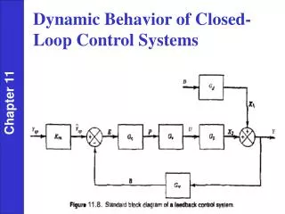
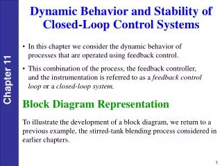
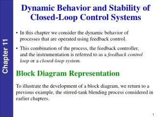
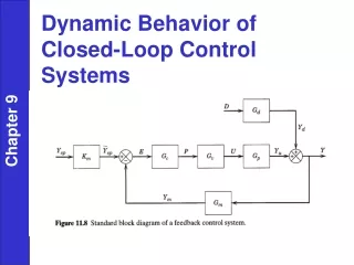
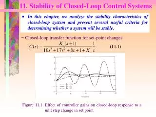
11. Stability of Closed-Loop Control Systems. In this chapter, we analyze the stability characteristics of closed-loop system and present several useful criteria for determining whether a system will be stable. - Closed-loop transfer function for set-point changes.

11. Stability of Closed-Loop Control Systems
E N D
Presentation Transcript
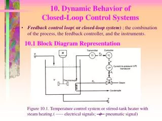
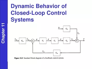
11. Stability of Closed-Loop Control Systems • In this chapter, we analyze the stability characteristics of closed-loop system and present several useful criteria for determining whether a system will be stable. - Closed-loop transfer function for set-point changes Figure 11.1. Effect of controller gains on closed-loop response to a unit step change in set point
11.1 General Stability Criterion • Open loop stable (Self-regulating) process: the stable process without feedback control • Definition of stability(BIBO Stability): An unconstrained linear system is said to be stable if the output response is bounded for all bounded inputs. Otherwise it is said to be unstable. Example Figure 11.2. A liquid storage system which is not self-regulating
Transfer function relating liquid level h to inlet flow rate qi For a step change of magnitude M0, Taking the inverse Laplace transform gives the transient response, Since this response is unbounded, we conclude that the liquid storage system is open-loop unstable (or non-self-regulating) since a bounded input has produced an unbounded response. However, if the pump in Fig.11.2 were replaced by a valve, then the storage system would be self-regulating.
11.1.1 Characteristic Equation In Chapter 10 where, GOL = GcGvGpGm For set-point changes, Eq. (11-5) reduces as where, m n for physical realizability From Eq. (11-6) the poles are also the roots of the following equation which is called as the characteristic equation: 1 + GOL = 0 plays a decisive role in determining system stability
If R(s) = 1/s and there are no repeated poles, then Thus, one of the poles is a positive real number, c(t) is unbounded. If pkis ak+jbk, imaginary part causes the oscillatory response and with a positive real part, then the system is unstable. • General Stability Criterion The conventional feedback control system is stable if and only if all roots of the characteristic equation are negative or have negative real parts. Otherwise, the system is unstable.
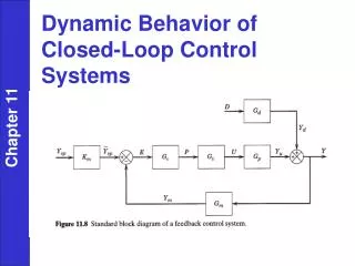
Figure 11.3. Stability regions in the complex plane for roots of the characteristic equation • Note) The same characteristic equation occurs for both load and set-point changes since the term, 1 + GOL. Thus, if the closed-loop system is stable for load disturbance, it will also be stable for set-point changes.
Figure 11.4. Contributions of characteristic equation roots to closed-loop response.
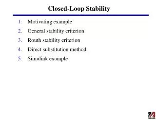
11.2 Routh Stability Criterion • Concept: an analytical technique for determining whether any roots of polynomial have positive real parts • Method: Characteristic Equation: ansn+ an-1sn-1+ ··· +a1s + a0 = 0 (an>0) 1) all the coefficients an , an-1, ··· a0 must be positive. (if any coefficient is negative or zero, then the system is unstable.) 2) construct Routh array
where, n is the order of characteristic equation, All of the elements in the left column of the Routh array are positive ⇒ only valid if characteristic equation is in polynomial of s (no time delay). ⇒ if system contain time delays use Pade approximation. Note) A exact stability analysis of system containing time delays will be treated in the frequency analysis.
11.3 Direct Substitution Method • Concept: Substituting s = jw into the characteristic equation → find a stability unit such as the maximum value of Kc . Example Use the direct-substitution method to determine Kcm for the system with the characteristic equation given by. 10s3 + 17s2 + 8s + 1 + Kc = 0 (11.9) Solution Substitute s = jw and Kc = Kcm into Eq.(11-9): -10jw3- 17w2 + 8jw + 1 + Kcm = 0 or (1 + Kcm- 17w2) +j(8w-10w3) = 0 (11.10) Equation (11.10) is satisfied if both real and imaginary parts of (11.10) are identically zero: 1 + Kcm- 17w2 = 0, 8w-10w3 = 0 Therefore, w = 0.894 Kcm = 12.6
Thus, we conclude that Kc < 12.6 for stability. • w = 0.894 indicates that at the stability limit (where Kc = Kcm = 12.6), a sustained oscillation occurs that has a frequency of w = 0.894 radians/min if the time constants have units of minutes. (Recall that a pair of complex roots on the imaginary axis, , results in an undamped oscillation of frequency w.) • The corresponding period P is P = 2p/0.894 = 7.03 min.
11.4 Root Locus Diagrams In the design and analysis of control systems, it is instructive to know how the roots of the characteristic equation change when a particular system parameter such as controller gain changes. • A root locus diagram provides a convenient graphical display of this information. Example) Consider a feedback control system that has the following open-loop transfer function. Plot the root locus diagram for 0 Kc 40
Solution: The C. E. is (s + 1)(s + 2)(s + 3) + 2Kc = 0. Figure 11.5. Root locus diagram for third-order system. From the above root locus diagram, • The closed-loop system is underdamped one for Kc > 0.2. • The closed-loop system is unstable for Kc > 30. • Disadvantage of root locus analysis. → cannot handle time delay. Thus, use the Pade approximation. → require iterative solution of the nonlinear and nonrational characteristic equation (but not easy).
Approximation by an underdamped second-order system. If the two closest roots are a complex conjugate pair, then the closed-loop system can be approximated by an under-damped second-order system. From C. E. These roots are shown in Fig. 11. 6 Figure 11.6. Root location for underdamped second-order system