Regression with a Binary Dependent Variable (SW Ch. 9)
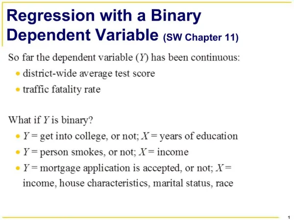
Regression with a Binary Dependent Variable (SW Ch. 9). So far the dependent variable ( Y ) has been continuous: district-wide average test score traffic fatality rate But we might want to understand the effect of X on a binary variable: Y = get into college, or not

Regression with a Binary Dependent Variable (SW Ch. 9)
E N D
Presentation Transcript
Regression with a Binary Dependent Variable(SW Ch. 9) So far the dependent variable (Y) has been continuous: • district-wide average test score • traffic fatality rate But we might want to understand the effect of X on a binary variable: • Y = get into college, or not • Y = person smokes, or not • Y = mortgage application is accepted, or not
Example: Mortgage denial and race The Boston Fed HMDA data set • Individual applications for single-family mortgages made in 1990 in the greater Boston area • 2380 observations, collected under Home Mortgage Disclosure Act (HMDA)
Variables • Dependent variable: • Is the mortgage denied or accepted? • Independent variables: • income, wealth, employment status • other loan, property characteristics • race of applicant
The Linear Probability Model (SW Section 9.1) A natural starting point is the linear regression model with a single regressor: Yi = 0 + 1Xi + ui But: • What does 1 mean when Y is binary? Is 1 = ? • What does the line 0 + 1X mean when Y is binary? • What does the predicted value mean when Y is binary? For example, what does = 0.26 mean?
The linear probability model, ctd. Yi = 0 + 1Xi + ui Recall assumption #1: E(ui|Xi) = 0, so E(Yi|Xi) = E(0 + 1Xi + ui|Xi) = 0 + 1Xi When Y is binary, E(Y) = 1×Pr(Y=1) + 0×Pr(Y=0) = Pr(Y=1) so E(Y|X) = Pr(Y=1|X)
The linear probability model, ctd. When Y is binary, the linear regression model Yi = 0 + 1Xi + ui is called the linear probability model. • The predicted value is a probability: • E(Y|X=x) = Pr(Y=1|X=x) = prob. that Y = 1 given x • = the predicted probability that Yi = 1, given X • 1 = change in probability that Y = 1 for a given x: 1 =
Example: linear probability model, HMDA data Mortgage denial v. ratio of debt payments to income (P/I ratio) in the HMDA data set (subset)
Linear probability model: HMDA data = -.080 + .604P/I ratio (n = 2380) (.032) (.098) • What is the predicted value for P/Iratio = .3? = -.080 + .604×.3 = .151 • Calculating “effects:” increase P/I ratio from .3 to .4: = -.080 + .604×.4 = .212 The effect on the probability of denial of an increase in P/I ratio from .3 to .4 is to increase the probability by .061, that is, by 6.1 percentage points (what?).
Next include black as a regressor: = -.091 + .559P/I ratio + .177black (.032) (.098) (.025) Predicted probability of denial: • for black applicant with P/I ratio = .3: =-.091+.559×.3+.177×1=.254 • for white applicant, P/I ratio = .3: = -.091+.559×.3+.177×0=.077 • difference = .177 = 17.7 percentage points • Coefficient on black is significant at the 5% level • Still plenty of room for omitted variable bias…
The linear probability model: Summary • Models probability as a linear function of X • Advantages: • simple to estimate and to interpret • inference is the same as for multiple regression (need heteroskedasticity-robust standard errors) • Disadvantages: • Does it make sense that the probability should be linear in X? • Predicted probabilities can be <0 or >1! • These disadvantages can be solved by using a nonlinear probability model: probit and logit regression
Probit and Logit Regression (SW Section 9.2) The problem with the linear probability model is that it models the probability of Y=1 as being linear: Pr(Y = 1|X) = 0 + 1X Instead, we want: • 0 ≤ Pr(Y = 1|X) ≤ 1 for all X • Pr(Y = 1|X) to be increasing in X (for 1>0) This requires a nonlinear functional form for the probability. How about an “S-curve”…
The probit model satisfies these conditions: • 0 ≤ Pr(Y = 1|X) ≤ 1 for all X • Pr(Y = 1|X) to be increasing in X (for 1>0)
Probit regression models the probability that Y=1 using the cumulative standard normal distribution function, evaluated at z = 0 + 1X: Pr(Y = 1|X) = (0 + 1X) • is the cumulative normal distribution function. • z = 0 + 1X is the “z-value” or “z-index” of the probit model. Example: Suppose 0 = -2, 1= 3, X = .4, so Pr(Y = 1|X=.4) = (-2 + 3×.4) = (-0.8) Pr(Y = 1|X=.4) = area under the standard normal density to left of z = -.8, which is…
Probit regression, ctd. Why use the cumulative normal probability distribution? • The “S-shape” gives us what we want: • 0 ≤ Pr(Y = 1|X) ≤ 1 for all X • Pr(Y = 1|X) to be increasing in X (for 1>0) • Easy to use – the probabilities are tabulated in the cumulative normal tables • Relatively straightforward interpretation: • z-value = 0 + 1X • + X is the predicted z-value, given X • 1 is the change in the z-value for a unit change in X
STATA Example: HMDA data = (-2.19 + 2.97×P/I ratio) (.16) (.47)
STATA Example: HMDA data, ctd. = (-2.19 + 2.97×P/I ratio) (.16) (.47) • Positive coefficient: does this make sense? • Standard errors have usual interpretation • Predicted probabilities: = (-2.19+2.97×.3) = (-1.30) = .097 • Effect of change in P/I ratio from .3 to .4: = (-2.19+2.97×.4) = .159 Predicted probability of denial rises from .097 to .159
Probit regression with multiple regressors Pr(Y = 1|X1, X2) = (0 + 1X1 + 2X2) • is the cumulative normal distribution function. • z = 0 + 1X1 + 2X2 is the “z-value” or “z-index” of the probit model. • 1 is the effect on the z-score of a unit change in X1, holding constant X2
STATA Example: HMDA data We’ll go through the estimation details later…
STATA Example: HMDA data, ctd. = (-2.26 + 2.74×P/I ratio + .71×black) (.16) (.44) (.08) • Is the coefficient on black statistically significant? • Estimated effect of race for P/Iratio = .3: = (-2.26+2.74×.3+.71×1) = .233 = (-2.26+2.74×.3+.71×0) = .075 • Difference in rejection probabilities = .158 (15.8 percentage points) • Still plenty of room still for omitted variable bias…
Logit regression Logit regression models the probability of Y=1 as the cumulative standard logistic distribution function, evaluated at z = 0 + 1X: Pr(Y = 1|X) = F(0 + 1X) F is the cumulative logistic distribution function: F(0 + 1X) =
Logistic regression, ctd. Pr(Y = 1|X) = F(0 + 1X) where F(0 + 1X) = . Example: 0 = -3, 1= 2, X = .4, so 0 + 1X = -3 + 2×.4 = -2.2 so Pr(Y = 1|X=.4) = 1/(1+e–(–2.2)) = .0998 Why bother with logit if we have probit? • Historically, numerically convenient • In practice, very similar to probit
Predicted probabilities from estimated probit and logit models usually are very close.
Estimation and Inference in Probit (and Logit) Models (SW Section 9.3) Probit model: Pr(Y = 1|X) = (0 + 1X) • Estimation and inference • How to estimate 0 and 1? • What is the sampling distribution of the estimators? • Why can we use the usual methods of inference? • First discuss nonlinear least squares (easier to explain) • Then discuss maximum likelihood estimation (what is actually done in practice)
Probit estimation by nonlinear least squares Recall OLS: • The result is the OLS estimators and In probit, we have a different regression function – the nonlinear probit model. So, we could estimate 0 and 1 by nonlinear least squares: Solving this yields the nonlinear least squares estimator of the probit coefficients.
Nonlinear least squares, ctd. How to solve this minimization problem? • Calculus doesn’t give and explicit solution. • Must be solved numerically using the computer, e.g. by “trial and error” method of trying one set of values for (b0,b1), then trying another, and another,… • Better idea: use specialized minimization algorithms In practice, nonlinear least squares isn’t used because it isn’t efficient – an estimator with a smaller variance is…
Probit estimation by maximum likelihood The likelihood function is the conditional density of Y1,…,Yn given X1,…,Xn, treated as a function of the unknown parameters 0 and 1. • The maximum likelihood estimator (MLE) is the value of (0, 1) that maximize the likelihood function. • The MLE is the value of (0, 1) that best describe the full distribution of the data. • In large samples, the MLE is: • consistent • normally distributed • efficient (has the smallest variance of all estimators)
Special case: the probit MLE with no X Y = (Bernoulli distribution) Data: Y1,…,Yn, i.i.d. Derivation of the likelihood starts with the density of Y1: Pr(Y1= 1) = p and Pr(Y1= 0) = 1–p so Pr(Y1 = y1) = (verify this for y1=0, 1!)
Joint density of (Y1,Y2): Because Y1 and Y2 are independent, Pr(Y1 = y1,Y2 = y2) = Pr(Y1 = y1) × Pr(Y2 = y2) = [ ] ×[ ] Joint density of (Y1,..,Yn): Pr(Y1 = y1,Y2 = y2,…,Yn = yn) = [ ] × [ ] × … × [ ] =
The likelihood is the joint density, treated as a function of the unknown parameters, which here is p: f(p;Y1,…,Yn) = The MLE maximizes the likelihood. Its standard to work with the log likelihood, ln[f(p;Y1,…,Yn)]: ln[f(p;Y1,…,Yn)] =