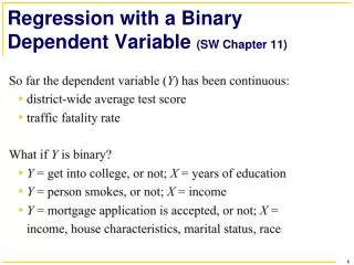
Regression with a Binary Dependent Variable (SW Chapter 11)
Regression with a Binary Dependent Variable (SW Chapter 11). Example: Mortgage denial and race The Boston Fed HMDA data set . The Linear Probability Model. The Linear Probability Model. Example : Linear Prob Model. Linear probability model: HMDA data. Linear probability model: HMDA data.


Regression with a Binary Dependent Variable (SW Chapter 11)
E N D
Presentation Transcript
Example: Mortgage denial and raceThe Boston Fed HMDA data set
Linear probability model: Application Cattaneo, Galiani, Gertler, Martinez, and Titiunik (2009). “Housing, Health, and Happiness.” American Economic Journal: Economic Policy 1(1): 75 - 105 • What was the impact of PisoFirme, a large-scale Mexican program to help families replace dirt floors with cement floors? • A pledge by governor Enrique Martinez y Martinez led to State of Coahuila offering free 50m2 of cement flooring ($150 value), starting in 2000, for homeowners with dirt floors
Cattaneo et al. (AEJ:Economic Policy 2009) “Housing, Health, & Happiness” X1 = “Program dummy” = 1 if offered Piso Firme.
Cattaneo et al. (AEJ:Economic Policy 2009) “Housing, Health, & Happiness” X1 = “Program dummy” = 1 if offered Piso Firme Interpretations?
Probit Regression Marginal Effects . sum pratio; Variable | Obs Mean Std. Dev. Min Max -------------+-------------------------------------------------------- pratio | 1140 1.027249 .286608 .497207 2.324675 . scalar meanpratio = r(mean); . sum disp_pepsi; Variable | Obs Mean Std. Dev. Min Max -------------+-------------------------------------------------------- disp_pepsi | 1140 .3640351 .4813697 0 1 . scalar meandisp_pepsi = r(mean); . sum disp_coke; Variable | Obs Mean Std. Dev. Min Max -------------+-------------------------------------------------------- disp_coke | 1140 .3789474 .4853379 0 1 . scalar meandisp_coke = r(mean); . probit coke pratio disp_coke disp_pepsi; Iteration 0: log likelihood = -783.86028 Iteration 1: log likelihood = -711.02196 Iteration 2: log likelihood = -710.94858 Iteration 3: log likelihood = -710.94858 Probit regression Number of obs = 1140 LR chi2(3) = 145.82 Prob > chi2 = 0.0000 Log likelihood = -710.94858 Pseudo R2 = 0.0930 ------------------------------------------------------------------------------ coke | Coef. Std. Err. z P>|z| [95% Conf. Interval] -------------+---------------------------------------------------------------- pratio | -1.145963 .1808833 -6.34 0.000 -1.500487 -.791438 disp_coke | .217187 .0966084 2.25 0.025 .027838 .4065359 disp_pepsi | -.447297 .1014033 -4.41 0.000 -.6460439 -.2485502 _cons | 1.10806 .1899592 5.83 0.000 .7357465 1.480373 ------------------------------------------------------------------------------
Predicted probabilities from estimated probit and logit models usually are (as usual) very close in this application.
Probit model: Application Arcidiacono and Vigdor (2010). “Does the River Spill Over? Estimating the Economic Returns to Attending a Racially Diverse College.” Economic Inquiry 48(3): 537 – 557. • Does “diversity capital” matter and does minority representation increase it? • Does diversity improve post-graduate outcomes of non-minority students? • College & Beyond survey, starting college in 1976
Logit model: Application Bodvarsson & Walker (2004). “Do Parental Cash Transfers Weaken Performance in College?” Economics of Education Review 23: 483 – 495. • When parents pay for tuition & books does this undermine the incentive to do well? • Univ of Nebraska @ Lincoln & Washburn Univ in Topeka, KS, 2001-02 academic year