Regression with Panel Data (SW Chapter 10)
Regression with Panel Data (SW Chapter 10). Outline. Panel Data: What and Why Panel Data with Two Time Periods Fixed Effects Regression Regression with Time Fixed Effects Standard Errors for Fixed Effects Regression Application to Drunk Driving and Traffic Safety. Panel Data: What and Why.


Regression with Panel Data (SW Chapter 10)
E N D
Presentation Transcript
Outline • Panel Data: What and Why • Panel Data with Two Time Periods • Fixed Effects Regression • Regression with Time Fixed Effects • Standard Errors for Fixed Effects Regression • Application to Drunk Driving and Traffic Safety
Panel Data: What and Why A panel dataset contains observations on multiple entities (individuals, states, companies…), where each entity is observed at two or more points in time. Hypothetical examples: • Data on 420 California school districts in 1999 andagain in 2000, for 840 observations total. • Data on 50 U.S. states, each state is observed in 3 years, for a total of 150 observations. • Data on 1000 individuals, in four different months, for 4000 observations total.
The Linear Probability Model (SW Section 9.1) Notation for panel data A double subscript distinguishes entities (states) and time periods (years) i = entity (state), n = number of entities, so i = 1,…,n t = time period (year), T = number of time periods, so t =1,…,T Data: Suppose we have 1 regressor. The data are: (Xit, Yit), i = 1,…,n, t = 1,…,T
Panel data notation, ctd. Panel data with k regressors: (X1it, X2it,…,Xkit, Yit), i = 1,…,n, t = 1,…,T n = number of entities (states) T = number of time periods (years) Some jargon… • Another term for panel data is longitudinal data • balanced panel: no missing observations, that is, all variables are observed for all entities (states) and all time periods (years)
Why are panel data useful? With panel data we can control for factors that: • Vary across entities but do not vary over time • Could cause omitted variable bias if they are omitted • Are unobserved or unmeasured – and therefore cannot be included in the regression using multiple regression Here’s the key idea: If an omitted variable does not change over time, then any changes in Y over time cannot be caused by the omitted variable.
Example of a panel data set:Traffic deaths and alcohol taxes Observational unit: a year in a U.S. state • 48 U.S. states, so n = # of entities = 48 • 7 years (1982,…, 1988), so T = # of time periods = 7 • Balanced panel, so total # observations = 7×48 = 336 Variables: • Traffic fatality rate (# traffic deaths in that state in that year, per 10,000 state residents) • Tax on a case of beer • Other (legal driving age, drunk driving laws, etc.)
U.S. traffic death data for 1982: Higher alcohol taxes, more traffic deaths?
U.S. traffic death data for 1988 Higher alcohol taxes, more traffic deaths?
Why might there be higher more traffic deaths in states that have higher alcohol taxes? Other factors that determine traffic fatality rate: • Quality (age) of automobiles • Quality of roads • “Culture” around drinking and driving • Density of cars on the road
Omitted variable bias. Example #1: traffic density. Suppose: • High traffic density means more traffic deaths • (Western) states with lower traffic density have lower alcohol taxes • Then the two conditions for omitted variable bias are satisfied. Specifically, “high taxes” could reflect “high traffic density” (so the OLS coefficient would be biased positively – high taxes, more deaths) • Panel data lets us eliminate omitted variable bias when the omitted variables are constant over time within a given state.
Omitted variable bias. Example #2: Cultural attitudes towards drinking and driving: • arguably are a determinant of traffic deaths; and • potentially are correlated with the beer tax. • Then the two conditions for omitted variable bias are satisfied. Specifically, “high taxes” could pick up the effect of “cultural attitudes towards drinking” so the OLS coefficient would be biased • Panel data lets us eliminate omitted variable bias when the omitted variables are constant over time within a given state.
Panel Data with Two Time Consider the panel data model, FatalityRateit = 0 + 1BeerTaxit + 2Zi + uit Zi is a factor that does not change over time (density), at least during the years on which we have data. • Suppose Zi is not observed, so its omission could result in omitted variable bias. • The effect of Zi can be eliminated using T = 2 years.
The key idea: Any change in the fatality rate from 1982 to 1988 cannot be caused by Zi, because Zi (by assumption) does not change between 1982 and 1988. The math: consider fatality rates in 1988 and 1982: FatalityRatei1988 = 0 + 1BeerTaxi1988 + 2Zi + ui1988 FatalityRatei1982 = 0 + 1BeerTaxi1982 + 2Zi + ui1982 Suppose E(uit|BeerTaxit, Zi) = 0. Subtracting 1988 – 1982 (that is, calculating the change), eliminates the effect of Zi…
FatalityRatei1988 = 0 + 1BeerTaxi1988 + 2Zi + ui1988 FatalityRatei1982 = 0 + 1BeerTaxi1982 + 2Zi + ui1982 so FatalityRatei1988 – FatalityRatei1982 = 1(BeerTaxi1988 – BeerTaxi1982) + (ui1988 – ui1982) • The new error term, (ui1988 – ui1982), is uncorrelated with either BeerTaxi1988 or BeerTaxi1982. • This “difference” equation can be estimated by OLS, even though Zi isn’t observed.
The omitted variable Zi doesn’t change, so it cannot be a determinant of the change in Y • This differences regression doesn’t have an intercept – it was eliminated by the subtraction step
Example: Traffic deaths and beer taxes 1982 data: = 2.01 + 0.15BeerTax (n = 48) (.15) (.13) 1988 data: = 1.86 + 0.44BeerTax (n = 48) (.11) (.13) Difference regression (n = 48) = –.072 – 1.04(BeerTax1988–BeerTax1982) (.065) (.36) An intercept is included in this differences regression allows for the mean change in FR to be nonzero – more on this later…
FatalityRate v. BeerTax: Note that the intercept is nearly zero…
Fixed Effects Regression (SW Section 10.3) What if you have more than 2 time periods (T > 2)? Yit = 0 + 1Xit + 2Zi + uit, i =1,…,n, T = 1,…,T We can rewrite this in two useful ways: • “n-1 binary regressor” regression model • “Fixed Effects” regression model We first rewrite this in “fixed effects” form. Suppose we have n = 3 states: California, Texas, and Massachusetts.
Yit = 0 + 1Xit + 2Zi + uit, i =1,…,n, T = 1,…,T Population regression for California (that is, i = CA): YCA,t = 0 + 1XCA,t + 2ZCA + uCA,t = (0 + 2ZCA) +1XCA,t + uCA,t or YCA,t = CA +1XCA,t + uCA,t • CA = 0 + 2ZCA doesn’t change over time • CA is the intercept for CA, and 1 is the slope • The intercept is unique to CA, but the slope is the same in all the states: parallel lines.
For TX: YTX,t = 0 + 1XTX,t + 2ZTX + uTX,t = (0 + 2ZTX) +1XTX,t + uTX,t or YTX,t = TX +1XTX,t + uTX,t, where TX = 0 + 2ZTX Collecting the lines for all three states: YCA,t = CA +1XCA,t + uCA,t YTX,t = TX +1XTX,t + uTX,t YMA,t = MA +1XMA,t + uMA,t or Yit = i + 1Xit + uit, i = CA, TX, MA, T = 1,…,T
In binary regressor form: • DC Ai = 1 if state is CA, = 0 otherwise. • DT Xi = 1 if state is TX, = 0 otherwise. • leave out DMAi (why?)
The regression lines for each state in a picture Y = CA + 1X Y Recall that shifts in the intercept can be represented using binary regressors… CA Y = TX + 1X CA Y = MA+ 1X TX TX MA MA X
Y = CA + 1X Y • In binary regressor form: • Yit = 0 + CADCAi + TXDTXi + 1Xit + uit • DCAi = 1 if state is CA, = 0 otherwise • DTXt = 1 if state is TX, = 0 otherwise • leave out DMAi (why?) CA Y = TX + 1X CA Y = MA+ 1X TX TX MA MA X
Summary: Two ways to write the fixed effects model • “n-1 binary regressor” form Yit = 0 + 1Xit + 2D2i + … + nDni + uit where D2i = , etc. • “Fixed effects” form: Yit = 1Xit + i + uit • i is called a “state fixed effect” or “state effect” – it is the constant (fixed) effect of being in state i
Fixed Effects Regression: Estimation Three estimation methods: • “n-1 binary regressors” OLS regression • “Entity-demeaned” OLS regression • “Changes” specification, without an intercept (only works for T = 2) • These three methods produce identical estimates of the regression coefficients, and identical standard errors. • We already did the “changes” specification (1988 minus 1982) – but this only works for T = 2 years • Methods #1 and #2 work for general T • Method #1 is only practical when n isn’t too big
1. “n-1 binary regressors” OLS regression Yit = 0 + 1Xit + 2D2i + … + nDni + uit (1) where D2i = , etc. • First create the binary variables D2i,…,Dni • Then estimate (1) by OLS • Inference (hypothesis tests, confidence intervals) is as usual (using heteroskedasticity-robust standard errors) • This is impractical when n is very large (for example if n = 1000 workers)
2. “Entity-demeaned” OLS regression The fixed effects regression model: Yit = 1Xit + i + uit The entity averages satisfy: = i + 1 + Deviation from entity averages: Yit – = 1 +
Entity-demeaned OLS regression, ctd. Yit – = + or = 1 + where = Yit – and = Xit – • and are “entity-demeaned” data • For i=1 and t = 1982, is the difference between the fatality rate in Alabama in 1982, and its average value in Alabama averaged over all 7 years.
Entity-demeaned OLS regression, ctd. = 1 + (2) where = Yit – , etc. • First construct the entity-demeaned variables and • Then estimate (2) by regressing on using OLS • This is like the “changes” approach, but instead Yit is deviated from the state average instead of Yi1. • Standard errors need to be computed in a way that accounts for the panel nature of the data set (more later) • This can be done in a single command in STATA
Example: Traffic deaths and beer taxes in STATA First let STATA know you are working with panel data by defining the entity variable (state) and time variable (year):
The panel data command xtreg with the option fe performs fixed effects regression. The reported intercept is arbitrary, and the estimated individual effects are not reported in the default output. • The fe option means use fixed effects regression • The vce(cluster state) option tells STATA to use clustered standard errors – more on this later
Example, ctd. For n = 48, T = 7: = –.66BeerTax + State fixed effects (.29) Should you report the intercept? • How many binary regressors would you include to estimate this using the “binary regressor” method? • Compare slope, standard error to the estimate for the 1988 v. 1982 “changes” specification (T = 2, n = 48) (note that this includes an intercept – return to this below): = –.072 – 1.04(BeerTax1988–BeerTax1982) (.065) (.36)
Regression with Time Fixed Effects(SW Section 10.4) An omitted variable might vary over time but not across states: • Safer cars (air bags, etc.); changes in national laws • These produce intercepts that change over time • Let St denote the combined effect of variables which changes over time but not states (“safer cars”). • The resulting population regression model is: Yit = 0 + 1Xit + 2Zi + 3St + uit
Time fixed effects only Yit = 0 + 1Xit + 3St + uit This model can be recast as having an intercept that varies from one year to the next: Yi,1982 = 0 + 1Xi,1982 + 3S1982 + ui,1982 = (0 + 3S1982) + 1Xi,1982 + ui,1982 = 1982 + 1Xi,1982 + ui,1982, where 1982 = 0 + 3S1982 Similarly, Yi,1983 = 1983 + 1Xi,1983+ ui,1983, where 1983 = 0 + 3S1983, etc.
Two formulations of regression with time fixed effects 1. “T-1 binary regressor” formulation: Yit = 0 + 1Xit + 2B2t + … TBTt + uit where B2t = , etc. 2. “Time effects” formulation: Yit = 1Xit + t + uit
Time fixed effects: estimation methods 1. “T-1 binary regressor” OLS regression Yit = 0 + 1Xit + 2B2it + … TBTit + uit • Create binary variables B2,…,BT • B2 = 1 if t = year #2, = 0 otherwise • Regress Y on X, B2,…,BT using OLS • Where’s B1? 2. “Year-demeaned” OLS regression • Deviate Yit, Xit from year (not state) averages • Estimate by OLS using “year-demeaned” data
Estimation with both entity and time fixed effects Yit = 1Xit + i + t + uit • When T = 2, computing the first difference and including an intercept is equivalent to (gives exactly the same regression as) including entity and time fixed effects. • When T > 2, there are various equivalent ways to incorporate both entity and time fixed effects: • entity demeaning & T – 1 time indicators (this is done in the following STATA example) • time demeaning & n – 1 entity indicators • T – 1 time indicators & n – 1 entity indicators • entity & time demeaning
First generate all the time binary variables • gen y83=(year==1983); • gen y84=(year==1984); • gen y85=(year==1985); • gen y86=(year==1986); • gen y87=(year==1987); • gen y88=(year==1988); • global yeardum "y83 y84 y85 y86 y87 y88";
The Fixed Effects Regression Assumptions and Standard Errors for Fixed Effects Regression • Under a panel data version of the least squares assumptions, the OLS fixed effects estimator of 1 is normally distributed. However, a new standard error formula needs to be introduced: the “clustered” standard error formula. This new formula is needed because observations for the same entity are not independent (it’s the same entity!), even though observations across entities are independent if entities are drawn by simple random sampling. • Here we consider the case of entity fixed effects. Time fixed effects can simply be included as additional binary regressors.
LS Assumptions for Panel Data Consider a single X: Yit = 1Xit + i + uit, i = 1,…,n, t = 1,…, T • E(uit|Xi1,…,XiT,i) = 0. • (Xi1,…,XiT,ui1,…,uiT), i =1,…,n, are i.i.d. draws from their joint distribution. • (Xit, uit) have finite fourth moments. • There is no perfect multicollinearity (multiple X’s) Assumptions 3&4 are least squares assumptions 3&4 Assumptions 1&2 differ
Assumption #1: E(uit|Xi1,…,XiT,i) = 0 • uit has mean zero, given the entity fixed effect and the entire history of the X’s for that entity • This is an extension of the previous multiple regression Assumption #1 • This means there are no omitted lagged effects (any lagged effects of X must enter explicitly) • Also, there is not feedback from u to future X: • Whether a state has a particularly high fatality rate this year doesn’t subsequently affect whether it increases the beer tax. • Sometimes this “no feedback” assumption is plausible, sometimes it isn’t. We’ll return to it when we take up time series data.
Assumption #2: (Xi1,…,XiT,ui1,…,uiT), i =1,…,n, are i.i.d. draws from their joint distribution. • This is an extension of Assumption #2 for multiple regression with cross-section data • This is satisfied if entities are randomly sampled from their population by simple random sampling. • This does not require observations to be i.i.d. overtime for the same entity – that would be unrealistic. Whether a state has a high beer tax this year is a good predictor of (correlated with) whether it will have a high beer tax next year. Similarly, the error term for an entity in one year is plausibly correlated with its value in the year, that is, corr(uit, uit+1) is often plausibly nonzero.
Autocorrelation (serial correlation) Suppose a variable Z is observed at different dates t, so observations are on Zt, t = 1,…, T. (Think of there being only one entity.) Then Zt is said to be autocorrelated or serially correlated if corr(Zt, Zt+j) ≠ 0 for some dates j ≠ 0. • “Autocorrelation” means correlation with itself. • cov(Zt, Zt+j) is called the jth autocovariance of Zt. • In the drunk driving example, uit includes the omitted variable of annual weather conditions for state i. If snowy winters come in clusters (one follows another) then uit will be autocorrelated (why?) • In many panel data applications, uit is plausibly autocorrelated.
Independence and autocorrelation in panel data in a picture: Sampling is i.i.d. across entities • If entities are sampled by simple random sampling, then (ui1,…, uiT) is independent of (uj1,…, ujT) for different entities i ≠ j. • But if the omitted factors comprising uit are serially correlated, then uit is serially correlated.