Introduction to Hidden Markov Models (HMMs)
420 likes | 436 Vues
This introduction covers probability, statistics, parameter estimation, hypothesis testing, and likelihood in the context of hidden Markov models. Learn about random variables, probability distributions, likelihood ratios, stochastic processes, and inference techniques. Discover the application of HMM in identifying patterns within sequences and making predictions based on hidden states.

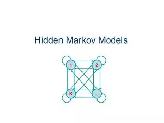
Introduction to Hidden Markov Models (HMMs)
E N D
Presentation Transcript
Introduction to Hidden Markov Models (HMMs) But first, some probability and statistics background
Random Variables and Probability Probability Distributions Parameter Estimation Hypothesis Testing Likelihood Conditional Probability Stochastic Processes Inference for Stochastic Processes Important Topics
Probability The probability of a particular event occurring is the frequency of that event over a very long series of repetitions. • P(tossing a head) = 0.50 • P(rolling a 6) = 0.167 • P(average age in a population sample is greater than 21) = 0.25
Random Variables A random variable is a quantity that cannot be measured or predicted with absolute accuracy.
Probability Distributions • The distribution of a random variable describes the possible values of the variable and the probabilities of each value. • For discrete random variables, the distribution can be enumerated; for continuous ones we describe the distribution with a function.
Examples of Distributions Binomial Normal
Parameter Estimation One of the primary goals of statistical inference is to estimate unknown parameters. For example, using a sample taken from the target population, we might estimate the population mean using several different statistics: the sample mean, the sample median, or the sample mode. Different statistics have different sampling properties.
Hypothesis Testing A second goal of statistical inference is testing the validity of hypotheses about parameters using sample data. If the observed frequency is much greater than 0.5, we should reject the null hypothesis in favor of the alternative hypothesis. How do we decide what “much greater” is?
Likelihood For our purposes, it is sufficient to define the likelihood function as Analyses based on the likelihood function are well-studied, and usually have excellent statistical properties.
We say that is the maximum likelihood estimate of . Maximum Likelihood Estimation The maximum likelihood estimate of an unknown parameter is defined to be the value of that parameter that maximizes the likelihood function:
If , then Some simple calculus shows that the MLE of is , the frequency of “successes” in our sample of size n. Example: Binomial Probability If we had been unable to do the calculus, we could still have found the MLE by plotting the likelihood:
Likelihood Ratio Tests Consider testing the hypothesis: The likelihood ratio test statistic is:
Distribution of the Likelihood Ratio Test Statistic Under quite general conditions, where n-1 is the difference between the number of free parameters in the two hypotheses.
The Parametric Bootstrap Why we need it: The conditions necessary for the asymptotic chi-squared distribution are not always satisfied. What it is: A simulation based approach for evaluating the p-value of a statistical test statistic (often a likelihood ratio)
Parametric Bootstrap Procedure • Compute the LRT using the observed data • Use the parameters estimated under the null hypothesis to simulate a new dataset of the same size as the observed data. • Compute the LRT for the simulated dataset. • Repeat steps 2 & 3, say, 1000 times. • Construct a histogram of the simulated LRTs. • The p-value for the test is the frequency of simulated LRTs that exceed the observed LRT.
Conditional Probability The conditional probability of event A given that event B has happened is
Stochastic Processes A stochastic process is a series of random variables measured over time. Values in the future typically depend on current values. • Closing value of the stock market • Annual per capita murder rate • Current temperature
ACGGTTACGGATTGTCGAA t = 0 ACaGTTACGGATTGTCGAA t = 1 ACaGTTACGGATgGTCGAA t = 2 ACcGTTACGGATgGTCGAA t = 3
Inference for Stochastic Processes We often need to make inferences that involve the changes in molecular genetic sequences over time. Given a model for the process of sequence evolution, likelihood analyses can be performed.
HMM: Hidden Markov Model • Does this sequence come from a particular “class”? • Does the sequence contain a beta sheet? • What can we determine about the internal composition of the sequence if it belongs to this class? • Assuming this sequence contains a gene, where are the splice sites?
Example: A Dishonest Casino • Suppose a casino usually uses “fair” dice (probability of any side is 1/6), but occasionally changes briefly to unfair dice (probability of a 6 is 1/2, all others have probability 1/10) • We only observe the results of the tosses • Can we identify the tosses with the biased dice?
The data we actually observe look like the following: 2 6 3 4 4 1 3 6 6 5 6 3 6 6 6 1 3 5 2 6 2 4 5 Which (if any) tosses were made using an unfair die? F F F F F F F F F F F F F F F F F F F F F F F F F F F F F U U U U F F U U U F F F F F F F F
2 6 3 4 4 1 3 6 6 5 6 3 6 6 6 1 3 5 2 6 2 4 5 F F F F F F F F F F F F F F F F F F F F F F F F F F F F F U U U U F F U U U F F F F F F F F If the tosses were made with a fair die (scenario 1), the probability of observing the series of tosses is: If the indicated tosses were made with an unfair die (scenario 2), then the series of tosses has probability The series of tosses is 87.5 times more probable under scenario 2 than under the scenario 1.
Transition Probabilities Emission Probabilities • 1/6 • 1/6 • 1/6 • 1/6 • 1/6 • 1/6 • 1/10 • 1/10 • 1/10 • 1/10 • 1/10 • 1/2 Hidden states 0.9 0.5 0.5 0.1 Fair Unfair
The Likelihood Function Probability of the data GIVEN the hidden states, in terms of 1 or more unknown parameters. Probability of the data in terms of 1 or more unknown parameters. Probability of the hidden states ( may depend on 1 or more unknown parameters). Compute via the forward algorithm
Predicting the Hidden States 1. The most probable state path (compute via the Viterbi algorithm): 2. Posterior state probabilities (compute via the backward algorithm):
Simple Gene Structure Model Start codon Stop codon 5’ UTR Exons Introns 3’ UTR
HMM Example: Gene Regions 5’ UTR 3’ UTR Exon Start Stop Intron
Content sensor: Region of residues with similar properties (introns, exons) Signal sensor: A specific signal sequence; might be a consensus sequence (start, stop codons)
E 5’ EI EF 3’ B S D A T F I ES Basic Gene-finding HMM • 5’: 5’ Untranslated region • EI: Initial exon • ES: Single exon • E: Exon • I: Intron • EF: Final exon • 3’: 3’ untranslated region • B: Begin Sequence • S: Start translation • D: Donor splice site • A: Acceptor splice site • T: Stop translation • F: End sequence
OK, What do we do with it now? The HMM must first be “trained” using a database of known genes. Consensus sequences for all signal sensors are needed. Compositional rules (i.e., emission probabilities) and length distributions are necessary for content sensors. Transition probabilities between all connected states must be estimated.
GENSCAN Chris Burge and Samuel Karlin J. Mol. Biol (1997) 268:78-94 Prediction of Complete Gene Structures in Human Genomic DNA
Basic features of GENSCAN • HMM description of human genomic sequences,including: • Transcriptional, translational, and splicing signals • Length distributions and compositional features of introns, exons, and intergenic regions • Distinct model parameters for regions with different GC compositions
Sn: Sensitivity = Prob(True nucleotide or exon predicted in a gene) Sp: Specificity = Prob(Predicted nucleotide or exon is in a gene) AC and CC are overall measures of accuracy, including both positive and negative predictions. ME: Prob(true exon is completely missed in the prediction) WE: Prob(predicted exon is not in a gene)
Profile HMMs A A C T - - C T A A T C T C - C G A A G C T - - T G G T G T T C T C T A A A C T C - C G A A G C T C - C G A PROSITE regular expression [AT][ATG][CT][T][CT]*[CT][GT][AG]
A A C T - - C T A A T C T C - C G A A G C T - - T G G T G T T C T C T A A A C T C - C G A A G C T C - C G A [AT][ATG][CT][T][CT]*[CT][GT][AG] T T T T T T T G The sequence matches the PROSITE expression at every position, but does it really “match” the profile?
0.25 A 0 C .75 G 0 T .25 0.6 0.75 A .8 C 0 G 0 T .2 A .8 C 0 G .2 T 0 A 0 C .8 G 0 T .2 A 0 C 0 G .6 T .4 A 0 C .8 G 0 T .2 A .4 C 0 G .4 T .2 A 0 C 0 G 0 T 1 1.0 1.0 1.0 0.4 1.0 1.0 A A C T - - C T A A T C T C - C G A A G C T - - T G G T G T T C T C T A A A C T C - C G A
0.25 A 0 C .75 G 0 T .25 0.6 0.75 A 0 C 0 G .6 T .4 A .8 C 0 G 0 T .2 A .4 C 0 G .4 T .2 A 0 C .8 G 0 T .2 A 0 C 0 G 0 T 1 A 0 C .8 G 0 T .2 A .8 C 0 G .2 T 0 1.0 1.0 1.0 0.4 1.0 1.0 T T T G T T T T T T T G T T T T
General Profile HMM Structure Delete States Dj Insert States Ij Match States Mj Begin End