Rotary Inverted Pendulum Balance Control
Rotary Inverted Pendulum Balance Control. Chengsen Song Dec. 1, 2010. Model. Non-linear Model. Modeling of the inverted pendulum system - Using Free Body Diagram method - Using Lagranian Formulation. State variables representation. Define the state variable x as

Rotary Inverted Pendulum Balance Control
E N D
Presentation Transcript
Rotary Inverted Pendulum Balance Control ChengsenSong Dec. 1, 2010
Non-linear Model Modeling of the inverted pendulum system - Using Free Body Diagram method - Using Lagranian Formulation
State variables representation • Define the state variable x as • Linearizing under the assumption that α ≈ 0, the state space representation of the pendulum is
Numerical solution • A = • 0 0 1.0000 0 • 0 0 0 1.0000 • 0 53.1012 -0.6586 0.6575 • 0 98.3814 -0.6575 1.2182 • B = • 0 • 0 • 274.4012 • 273.9627 • C = • 1 0 0 0 • 0 1 0 0 • D = • 0 • 0 • eig(A)= • 0 • 10.3650 • -9.5021 • -0.3033
K • Gain K is decided by the LQR controller design method. • LQR : determine the matrix gain K such that the static, full-state feedback control law u(t) = −Kx(t) satisfies the following criteria • a) the closed-loop system is asymptotically stable • b) the quadratic performance functionalis minimized • x = 10; • y = 500; • Q = [x 0 0 0; • 0 y 0 0; • 0 0 0 0; • 0 0 0 0]; • R = 15; • Klqr = lqr(A,B,Q,R)
L • Matrix Lis decided using the pole placement method. • Given the single- or multi-input system and a vector p of desired self-conjugate closed-loop pole locations, place computes a gain matrix K such that the state feedback u = –Kx places the closed-loop poles at the locations p. • P = [-2 -5 -42 -43]; • L = place(A',C',P)';
N • Gain N is to eliminate the steady-state error. • Cn = [1 0 0 0]; • sys = ss(A,B,Cn,0); • Nbar = rscale(sys,Klqr)
Future goal • Digital control system. • Varying sampling time. • Delay analysis