Wind-Driven Closed Gyre Circulation: A Quasi-Geostrophic Approach
Explore the vorticity balance in homogeneous fluid, quasi-geostrophic vorticity equation, Stommel and Munk models, boundary layers, and numerical results in closed gyre circulation models. Delve into non-dimensional equations, Rossby and Ekman numbers, western intensification, and dynamics in boundary layers.


Wind-Driven Closed Gyre Circulation: A Quasi-Geostrophic Approach
E N D
Presentation Transcript
Wind Driven Circulation III • Closed Gyre Circulation • Quasi-Geostrophic Vorticity Equation • Westward intensification • Stommel Model • Munk Model • Inertia boundary layer • Numerical results • Observations
Consider the vorticity balance of an homogeneous fluid (=constant) on an f-plane
Assume geostrophic balance on -plane approximation, i.e., ( is a constant) Vertically integrating the vorticity equation barotropic we have The entrainment from bottom boundary layer The entrainment from surface boundary layer We have where
Quasi-geostrophic vorticity equation and , we have For and where (Ekman transport is negligible) Moreover, We have where
Posing the gyre problem Boundary conditions on a solid boundary L (1) No penetration through the wall (2) No slip at the wall
Consider a homogeneous fluid on a -plane Non-dimensional Equation, An Example Define the following non-dimensional variables: (geostrophy) By definition
Define the non-dimensional parameters Rossby Number Horizontal Ekman Number Ekman depth Vertical Ekman Number Then, we have (with prime dropped) The solution
In the interior of the ocean, Eh<<1 and Ez<<1 (geostrophy) Near the bottom or surface, Ez≈O(1) In the surface and bottom boundary layers, the vertical scales are redefined (shortened, a general character of a boundary layer)
Non-dmensional vorticity equation Non-dimensionalize all the dependent and independent variables in the quasi-geostrophic equation as where For example, The non-dmensional equation where , nonlinearity. , , , bottom friction. , lateral friction. ,
Interior (Sverdrup) solution If <<1, S<<1, and M<<1, we have the interior (Sverdrup) equation: (satistfying eastern boundary condition) (satistfying western boundary condition) Example: Let , . Over a rectangular basin (x=0,1; y=0,1)
Westward Intensification It is apparent that the Sverdrup balance can not satisfy the mass conservation and vorticity balance for a closed basin. Therefore, it is expected that there exists a “boundary layer” where other terms in the quasi-geostrophic vorticity is important. This layer is located near the western boundary of the basin. Within the western boundary layer (WBL), , for mass balance The non-dimensionalized distance is , the length of the layer δ <<L In dimensional terms, The Sverdrup relation is broken down.
The Stommel model Bottom Ekman friction becomes important in WBL. , S<<1. at x=0, 1; y=0, 1. No-normal flow boundary condition (Since the horizontal friction is neglected, the no-slip condition can not be enforced. No-normal flow condition is used). Interior solution
Re-scaling in the boundary layer: , we have Let Take into As =0, =0. As ,I
The solution for is , . A=-B , ( can be the interior solution under different winds) For , , . For , , .
The dynamical balance in the Stommel model In the interior, Vorticity input by wind stress curl is balanced by a change in the planetary vorticity f of a fluid column.(In the northern hemisphere, clockwise wind stress curl induces equatorward flow). In WBL, , Since v>0 and is maximum at the western boundary, the bottom friction damps out the clockwise vorticity. Question: Does this mechanism work in a eastern boundary layer?