Wind-driven Ocean Circulation (steady state)
Wind-driven Ocean Circulation (steady state). Winds do NOT drive ocean currents, but the “ torque ” or “ spin ” or “ curl ” or “ vorticity ”

Wind-driven Ocean Circulation (steady state)
E N D
Presentation Transcript
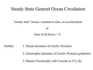
Wind-driven Ocean Circulation (steady state) Winds do NOT drive ocean currents, but the “torque” or “spin” or “curl” or “vorticity” provided by a spatially variable wind field drives large scale ocean circulations consisting of basin-wide gyres and western boundary currents within the surface 1000-m of all the world’s oceans. Need: 1. Ekman dynamics (Coriolis~Friction) 2. Geostrophic dynamics (Coriolis~Pressure gradients) 3. Ekman+Geostrophy with Coriolis as f=f0+by
Summary: Wind-stress curl (spin or vorticity) imparted by the wind) drives ocean circulation NOT the wind y, north Wind-curl = 0 Wind-curl<0 Wind-curl=0 x, east Ocean gyres are defined by where this “curl” is zero Each ocean gyre has a strong western boundary current Conservation of potential vorticity (spin) explains ocean circulation well
Atlantic surface circulation (adjusted steric height)(Reid, 1994) Note: Subtropical gyres (anticyclonic) Subpolar gyres (cyclonic) Note: westward intensification of the currents - strong currents are all on the western boundary, regardless of hemisphere Adapted from Talley (2008)
Schematic of surface circulation (Schmitz, 1995) Why are there gyres? Why are the currents intensified in the west? (“western boundary currents”) Adapted from Talley (2008)
westerlies trades = LAND Observed asymmetry of wind-driven gyres what one might expect what one observes (Stommel figures for circulation assuming perfect westerlies and trades) WHY? Adapted from Talley (2008)
vertical integral X-momentum: Coriolis = pressure gradient + friction Y-momentum: Coriolis = pressure gradient -rfv = -∂p/∂x + ∂t(x)/∂z -f M(y) = -∂P/∂x + t(x) rfu = -∂p/∂y f M(x) = -∂P/∂y y, north Zonal winds t(x) (y) x, east
-f ME(y) = t(x) -f Mg(y) = -∂P/∂x f ME(x) = 0 f Mg(x) = -∂P/∂y Separate M = Mekman+Mgeostrophic=ME+Mg: X-momentum: Y-momentum: Ekman geostrophic Ekman flux divergence ∂ME(x)/∂x + ∂ME(y)/∂y gives ∂ME(x)/∂x = 0 and ∂ME(y)/∂y = -∂(t(x) /f)/∂y = [-∂t(x)/∂y + bt(x)/f]/f = [-∂t(x)/∂y - bME(y)]/f b=∂f/∂y
div(ME) = -ME(y)b/f - (∂t(x)/∂y)/f div(Mg) = -Mg(y)b/f 0 = -M(y)b - ∂t(x)/∂y + M(y) = -1/b ∂t(x)/∂y Sverdrup’s relation Now for continuity div(M) = ∂M(x) /∂x + ∂M(y) /∂y gives or The total (Ekman plus geostrophic) mass flux in the north-south direction is equal to the wind stress “curl” or “torque” divided by the gradient of the Coriolis parameter with latitude
M(y) = -1/b ∂t(x)/∂y Sverdrup’s relation What about the east-west total flux M(x)? Calculate from continuity, e.g., ∂M(x)/∂x + ∂M(y)/∂y = 0 via integration across the ocean basin M(x) = - ∫ ∂M(y)/∂y dx
Sverdrup transport solution for observed annual mean wind field ∂t(x)/∂y=0 Ocean “gyres” are defined by contours of zero wind stress curl Reid (1948) Adapted from Stewart (2005)
Figure 11.2 Mass transport in the eastern Pacific calculated from Sverdrup’s theory using observed winds (solid lines) and pressure calculated from hydrographic data from ships. Transport is in tons per second through a section one meter wide extending from the sea surface to a depth of one kilometer. Note the difference in scale between My and Mx. From Reid (1948). Adapted from Stewart (2005)
Figure 11.3 Depth-integrated Sverdrup transport applied globally using the wind stress from Hellerman and Rosenstein (1983). Contour interval is 10 Sverdrups. From Tomczak and Godfrey (1994). Adapted from Stewart (2005)
Sverdrup assumed: i) The internal flow in the ocean is geostrophic; ii) there is a uniform depth of no motion; and iii) Ekman's transport is correct. The solutions are limited to the east side of the oceans because M(x) grows with x. The result stems from neglecting friction which would eventually balance the wind-driven flow. Nevertheless, Sverdrup solutions have been used for describing the global system of surface currents. The solutions are applied throughout each basin all the way to the western limit of the basin. There, conservation of mass is forced by including north-south currents confined to a thin, horizontal boundary layer. Only one boundary condition can be satisfied, no flow through the eastern boundary. More complete descriptions of the flow require more complete equations. The solutions give no information on the vertical distribution of the current. Results were based on data from two cruises plus average wind data assuming a steady state. Later calculations by Leetma, McCreary, and Moore (1981) using more recent wind data produces solutions with seasonal variability that agrees well with observations provided the level of no motion is at 500m. If another depth were chosen, the results are not as good. Adapted from Stewart (2005)
How does Ekman upwelling and downwelling affect the ocean below the Ekman layer?Step 1: Define Vorticity and potential vorticity Vorticity > 0 (positive) Vorticity < 0 (negative) Adapted from Talley (2008)
Potential vorticity CONSERVED, like angular momentum, but applied to a fluid instead of a solid Potential vorticity Q = (f + )/Hhas three parts: 1. Vorticity (“relative vorticity” ) due to fluid circulation 2. Vorticity (“planetary vorticity” f) due to earth rotation, depends on local latitude when considering local vertical column 3. Stretching 1/H due to fluid column stretching or shrinking The two vorticities (#1 and #2) add together to make the total vorticity = f + . The stretching (height of water column) is in the denominator since making a column taller makes it spin faster and vice versa. Potential vorticity Q = (relative + planetary vorticity)/(column height) Adapted from Talley (2008)
Conservation of potential vorticity (relative plus planetary) Conservation of potential vorticity (relative and stretching) Potential vorticity Adapted from Talley (2008)
Potential vorticity Conservation of potential vorticity (planetary and stretching) This is the potential vorticity balance for Sverdrup transport (next slide) Adapted from Talley (2008)
Ekman transport convergence and divergence Ekman Pumping Geostrophic flow Vertical velocity at base of Ekman layer: order (10-4cm/sec) (Compare with typical horizontal velocities of 1-10 cm/sec) Adapted from Talley (2008)
Sverdrup transport • Ekman pumping provides the squashing or stretching. • The water columns must respond. They do this by changing latitude. • (They do not spin up in place.) Q=f/H H here is the layer below thermocline Squashing -> equatorward movement Stretching -> poleward Adapted from Talley (2008)
How does Ekman transport drive underlying circulation?Step 2: Potential vorticity and Sverdrup transport Q = (f + )/H Sverdrup transport: If there is Ekman convergence (pumping downward), then H in the potential vorticity is decreased. This must result in a decrease of the numerator, (f + ). Since we know from observations (and “scaling”) that relative vorticity does not spin up, the latitude must change so that f can change. If there is a decrease in H, then there is a decrease in latitude - water moves towards the equator. Sverdrup transport = meridional flow due to pumping/suction Adapted from Talley (2008)
Western boundary currents: the return flow for the interior Sverdrup transport • WBCs must remove the vorticity put in by the wind • E.g. Ekman downwelling: wind puts in negative vorticity • E.g. WBC for downwelling gyre must put in positive vorticity From Ocean Circulation (Open University Press)
Western boundary currents: Gulf Stream as an example from sea surface temperature (satellite) and Benjamin Franklin’s map SST satellite image, from U. Miami RSMAS Richardson, Science (1980) Adapted from Talley (2008)
Gulf Stream velocity section in Florida Strait Roemmich, JPO ( 1983)
Western boundary currents Adapted from Talley (2008)
Summary: Wind-stress curl (spin or vorticity) imparted by the wind) drives ocean circulation NOT the wind y, north Wind-curl = 0 Wind-curl<0 Wind-curl=0 x, east Ocean gyres are defined by where this “curl” is zero Each ocean gyre has a strong western boundary current Conservation of potential vorticity (spin) explains ocean circulation well
X-momentum Y-momentum -rfv = -∂p/∂x + ∂t(x)/∂z -f M(y) = -∂P/∂x + t(x) rfu = -∂p/∂y + ∂t(y)/∂z f M(x) = -∂P/∂y + t(y) ∫ • dz Separate M = Mekman+Mgeostrophic=ME+Mg: -f ME(y) = t(x) -f Mg(y) = -∂P/∂x f ME(x) = t(y) f Mg(x) = -∂P/∂y Now for continuity div(M) = ∂M(x)/∂x + ∂M(y) gives div(ME) = -ME(y)b/f + (∂t(y)/∂x- ∂t(x)/∂y)/f div(Mg) = -Mg(y)b/f 0 = -M(y)b + curl t +
X-momentum Y-momentum -rfv = -∂p/∂x + ∂t(x)/∂z -f M(y) = -∂P/∂x + t(x) rfu = -∂p/∂y f M(x) = -∂P/∂y ∫ • dz Separate M = Mekman+Mgeostrophic=ME+Mg: -f ME(y) = t(x) -f Mg(y) = -∂P/∂x f ME(x) = 0 f Mg(x) = -∂P/∂y Now for continuity div(M) = ∂M(x)/∂x + ∂M(y) gives div(ME) = -ME(y)b/f - (∂t(x)/∂y)/f div(Mg) = -Mg(y)b/f 0 = -M(y)b - ∂t(x)/∂y +