Download
1 / 20
200 likes | 225 Vues
Workshop on utilizing multispectral infrared satellite data to simulate surface emissivity for radiative transfer modeling of the atmosphere. This includes fitting hyperspectral library data, extracting soil emissivities, and producing continuous sampled spectra. Contrast ratios, spectral shapes, and emissivity differences between MODIS and library data are analyzed for physical applications. DARPA research on spectral contrast and soil disturbance is discussed. Seasonal emissivity products and dynamic simulation based on geographically defined pixels are also explored. Planned work includes delivery in April 2005.

E N D
Surface Characterization 4th Annual Workshop on Hyperspectral Meteorological Science of UW MURI And Beyond Donovan Steutel Paul G. Lucey University of Hawai‘i
Provide emissivity boundary condition for radiative transfer modeling of atmosphere Use multispectral infrared satellite data as base map Fit infrared multispectral data with hyperspectral library data Produce continuous sampled spectrum at each pixel Surface Emissivity Simulation
MODIS features several bands with weak atmospheric extinction appropriate for surface characterization
MODIS team generates emissivity models for cloud-purged mosaics False color MODIS image
Extract soil emissivities at MODIS wavelengths (assuming Kirchoff’s Law) from ASTER spectrum library (41 soils) Treat ASTER soils as lookup table Compare each MODIS spectrum to lookup table and return soil sample# for closest fit (by RMS differences) Insert full resolution ASTER spectrum at each location Emissivity assignment
Mean-normalized comparison Difference of library match 0% 1.5% 3%
Absolute emissivity comparison Emissivity difference after gain/offset 0% 0.75% 1.5%
MODIS Emissivity Type Map Spatial resolution: 0.05° (~5km at equator) Wavelength range: 685-2250 cm-1 Wavelength sampling: 2 cm-1 Spectral channels: 801 White dune sand stony coarse sand Coniferous vegetation Deciduous vegetation Grass Other No data
Contrast ratios between library and MODIS spectra with similar spectral shapes can achieve large values routinely. Is this physical?
DARPA research conducted by the University of Hawai‘i [Johnson et al., 1998] discovered a consistent difference in spectral contrast associated with soil disturbance: Sampled sites have lower spectral contrast than surfaces measured in the field.
Disturbed location Background soil Solid is ground truth data Symbols are airborne hyperspectral data1
If particle sizes are less than the attenuation scale, partial coupling is enabled because of incomplete damping. This leads to higher emissivity and lower reflectance of small particles. (Gold blacks exploit this phenomenon in the visible). LWIR Observable Quartz. Particles >75 microns show high reflectance at 9 microns. Sample containing large amounts of fine particles show low reflectance
“Clean” Dirt (unsampled) “Dirty” Dirt (sampled)
Particles in the size range of 1-10 microns are very abundant in natural soils leading, and their abundance is coupled to natural geologic processes. This leads to relatively large variations in spectral contrast Sampled soils show low spectral contrast relative to the surroundings, as well as lower variation in contrast. This is consistent with an enhanced abundance of small particles. Conclusion: High contrast ratios are physical, but need further investigation in individual cases Library vs. MODIS emissivity contrast
Seasonal emissivity products Dec. 2002 MOD11C3 Dec. 2002 monthly average, 0.05° scale Model inputs may be dynamic to account for temporal variations in emissivity
Seasonal emissivity products Aug. 2003 MOD11C3 Aug. 2003 monthly average, 0.05° scale Model inputs may be dynamic to account for temporal variations in emissivity
Seasonal emissivity products Oct. 2003 MOD11C3 Oct. 2003 monthly average, 0.05° scale Model inputs may be dynamic to account for temporal variations in emissivity
Assign hyperspectral signatures to each geographically defined pixel for each season From seasonal data produce a dynamic emissivity simulation to include vegetation senescence effects MOD11C series available daily (C1), 8-day (C2), and monthly (C3) Delivery of this product: April 2005 Planned work