Analyzing Orbit Response Measurements for SPS and LHC: Techniques and Software Overview
160 likes | 301 Vues
This summary presents insights into orbit response analysis from SPS and its implications for LHC operations. The orbit response matrix connects changes in monitor positions to steering magnet deflections, enabling precise trajectory adjustments. A step-by-step methodology is outlined for preparing measurements, adjusting response data, and utilizing software tools like LOCO and MADX. Real case studies from SPS are highlighted, showcasing calibration challenges, fitting durations, and the impact of non-linear effects. This work underlines the necessity of meticulous calibrations in collider settings.

Analyzing Orbit Response Measurements for SPS and LHC: Techniques and Software Overview
E N D
Presentation Transcript
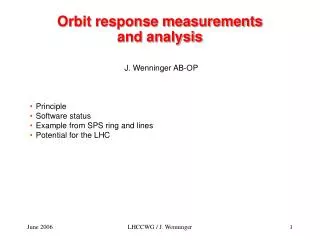
Orbit response measurementsand analysis • J. Wenninger AB-OP • Principle • Software status • Example from SPS ring and lines • Potential for the LHC LHCCWG / J. Wenninger
Orbit response • The orbit or trajectory response matrix relates the position change at monitors to the deflection at steering magnets (usually orbit correctors). • The position change Dui @ ith monitor is related to a kick qj @ jth corrector by : R = response matrix • In a linear approximation : Closed orbit Trajectory LHCCWG / J. Wenninger
Orbit response – remarks • R does not provide direct information on the optical functionb, m, …: • Step 1 : the measured R must be adjusted to match the model. • Step 2 : the optical functions are obtained from the matched model. • In a transfer line it is not possible to determine the optical functions since they depend on the initial conditions. The R matrix only provides information on the what happens within the line. But it gives indications the correctness of the line settings. • The measured R also depends on the BPM and corrector calibrations: • complicates fits, in particular CBP may depend on amplitude ! • R is not limited to linear effects, at large enough amplitudes non-linear effect can potentially be observed. Coupling may be included in a straightforward way. LHCCWG / J. Wenninger
Response matrix fits • Data preparation : • A vector holding the weighted difference between the measured and modeled response is build from all matrix elements : s is the measurement error • 2) Local gradient : • Evaluate the sensitivity wrt parameters c1 to cn(BPM and corrector calibrations, strengths…). • Straightforward for calibrations, requires MADX runs for model parameters (quad strengths…) linear approximation. LHCCWG / J. Wenninger
Response matrix fits (II) 3) Least-square minimization : Solve the linearised equation for parameter changes Dc (based on SVD). 4) Iteration : Update c, update G, solve again… until the solution is stable. m = # elements Rij LHCCWG / J. Wenninger
Matrix sizes… For a ring /line with N BPMs and M correctors per plane, the minimum size of the gradient matrix G is : (2 N M) (2 (N + M)) …with only BPM and corrector calibrations as parameters for c. • SPS transfer line : N < 30, M < 30 1800 x 120 0.2 x 10⁶ elements • SPS ring : N ~ 110 , M = 108 25000 x 220 6 x 10⁶ elements • LHC : N ~ 500 , M ~ 250 250000 x 1500 375 x 106 elements • The complete LHC is tough to handle with all elements included : RAM + precision + CPU time LHCCWG / J. Wenninger
Software… • The fit program I use at the SPS is a based on the LOCO program by J. Safranek: • Adapted to MADX + CERN/SPS environment (for example single plane BPMs, IO, …). • Display of results with PAW macros (to be moved to root this year). • Automatized response measurements are provided by the new steering SW in LSA. Data ‘transfer’ raw data LOCO through a small interface program. • I use it for: • SPS ring (since 2002) • TT10 (since 2006) • TT40/TI8 (since 2003) • CNGS (ready to go for commissioning run) • (Simple) results can be available online for transfer lines (few minutes). • For example TI8: results at ~01:00 AM less than 15 minutes after data taking… but nobody to watch because everyone else had left ! • Running the program requires ‘my presence’ – this is not a program that can be run blindly by anyone. And I have no plans to change this… LHCCWG / J. Wenninger
‘Time performance’ • Example for fit duration for some real cases. • SPS ring, 110 BPMs: • 10-20 correctors, fit calibrations factors and main quad strengths. • 10-30 minutes (P4) • 20 correctors, fit all (!!) 216 quadrupole strengths. many hours (I can’t remember !). • TI8, TT10, CNGS, all correctors and all BPMs : • fit calibrations and some strengths (2-5) less than 5 minutes (P4) • identify small coupling sources (TI8) many hours, multiple iterations and manual interventions LHCCWG / J. Wenninger
SPS example : before fit Since the SPS lattice is very simple, the model tune is set far away (0.2) from the actual tune in the example to make life a bit more difficult for the fit. Response for a horizontal and a vertical corrector (1% of the matrix). (*) + line : model Histogram : raw data MDHD.118 MDV.121 LHCCWG / J. Wenninger
SPS example : a few fit iterations later… Details on SPS results can be found in CERN-AB-2004-009 • BPM and correctors are calibrated. • Fitted model tunes exactly as expected ! • Excellent agreement model-data. (*) + line : fit model (17 MAD parameters) with calibrated kick Histogram : gain corrected data Empty bin BPM rejected MDHD.118 MDV.121 LHCCWG / J. Wenninger
TI8 example : quadrupole with wrong setting Details on TI8 results can be found in AB-Note-2006-021 • Initial measurement : • First H corrector data does not fit the line model when only main QD/QF strengths are allowed as free parameters. • Fitting one additional quad at a time, the fit gives a consistent/reasonable result only for DK/K = -20% on QTLF4004. Increase of QTLF4004 strength by 20% restores the model.. Histogram : data * + Line : model fit LHCCWG / J. Wenninger
TI8 example : arc cell phase advance • The TI8 arc cells have a nominal phase advance of 90 degrees (~SPS cells). • To obtain a good fit to the data the strength of the vertical QD family had to be increased by 1%. • clearly visible on the plots below : in the V plane the phase slips… • Since in the LHC the BPM sampling is four times higher than for TI8, this reveals an interesting potential for optics checks even before establishing a closed orbit ! Histogram : data * + Line : model fit H plane V plane LHCCWG / J. Wenninger
TT10 example : strong coupling Horizontal kick H plane • The SPS injection line TT10 is fully coupled when we run fixed target beam to exchange the planes (related to PS beam emittance and SPS aperture). • LOCO is perfectly able to handle this line. In fact the model matches the data perfectly (down to the BPM noise of 0.3 mm) without any adjustment (June 2006). Skew quad section - the excursion flips to the V plane V plane LHCCWG / J. Wenninger
LHC case : first turn (even after closed orbit established…) • Polarity errors are detected very easily (dipole correctors, quadrupoles, BPMs). • BPM errors. • Strength errors can be detected and identified down to a few%, provided they are isolated (i.e. not 5 in a row… - then only detection). Note that fits in that case need some guidance (to avoid having to many free parameters). The fact that measurements with correctors downstream of an error are not affected helps to localize problems when they are ‘difficult’ to understand. • Average phase advance over an arc could be measured to the permill level. • b3 may be observed if the BPMs are performing well – see LHC Project Note 314. LHCCWG / J. Wenninger
LHC case : closed orbit • BPM quality and calibrations.Measurements require only 4-20 correctors/plane/ring, selected to sample all phases – makes the fit manageable. • Correctors calibrations (and polarity). At least one complete data set with all correctors must be made for a complete check (first turn trajectory or closed orbit). • Optics : response fits can do a lot, but the fits are heavy! • Linear optics :for me phase advance measurements are ‘lighter’ and faster (fit) – For that reason I have also developed in 2004 a fit program (similar to R. Thomas) for the phase advance, interfaced to the SPS multi-turn acquisition program (also my baby). Synergy possible with R. Thomas’ stuff, since he did not seem ready to write SW… • Non-linear optics : there may be a potential here with ‘large amplitude’ kicks – to be checked. Note that I tried to see non-linear fields at the SPS with amplitudes of 30 mm (H plane), but the BPM uncertainties (non-linearity I guess) seemed to dominate the expected signals. LHCCWG / J. Wenninger
Conclusions • Response measurements and their analysis have proven to be very useful at the SPS. Various effects (not all were presented here) have been uncovered. And there is more to come with CNGS. • The SW chain is well tested and in place – including automated data acquisition. • Response measurements will obviously be made at the LHC to calibrate BPMs and orbit correctors – requires only small data samples. • Linear optics • This method has the highest potential with the trajectory / first turn, i.e. for early debugging. In particular because the SW chain itself is well tested – an asset during commissioning. • Phase advance measurements are much better once the closed orbit is established. • Non-linear optics may be an area where this method could be powerful – but we need very well understood BPMs. LHCCWG / J. Wenninger
