Understanding Machine Learning: Key Concepts and Techniques in Supervised and Unsupervised Learning
This summary covers essential concepts in machine learning, focusing on supervised and unsupervised learning. It introduces basic terminology like learners, algorithms, parameters, and models, highlighting the importance of tuning parameters with training sets and assessing generalization using test sets. It discusses the importance of feature selection and extraction for dimensionality reduction, the bias-variance tradeoff, and the concept of overfitting. Additionally, it offers insights into error metrics such as MSE and RMS to evaluate model performance.


Understanding Machine Learning: Key Concepts and Techniques in Supervised and Unsupervised Learning
E N D
Presentation Transcript
Basic terminology • tasks • classification • regression • learner, algorithm • each has one or several parameters influencing its behavior • model • one concrete combination of learner and parameters • tune the parameters using the training set • the generalization is assessed using test set (previously unseen data)
learning (training) • supervised • a target vectort is known, parameters are tuned to achieve the best match between prediction and the target vector • unsupervised • training data consists of a set of input vectors x without any corresponding target value • clustering, vizualization
for most applications, the original input variables must be preprocessed • feature selection • feature extraction x784 x6 x5 x4 x3 x2 x1 x1 x2 x3 x4 x5 x6 x784 ... ... selection extraction x1 x5 x456 x103 x*1 x*2 x*3 x*4 x*5 x*6 x*784 ... x*18 x*152 x*309 x*666
feature selection/extraction = dimensionality reduction • generally good thing • curse of dimensionality • example: • learner: regression (polynomial, y = w0 + w1x + w2x2 + w3x3 + …) • parameters: weights (coeffiients) w, order of polynomial • weights • adjusted so the the sum of squared errors SSE (error function) is as small as possible suma čtverců chyb predicted known target
Model selection overfitting
RMS – root mean squared error odmocninastřední kvadratické chyby MSE – mean squared error střední kvadratická chyba comparing error for data sets of different size – root mean squared errorRMS
Summary of errors sum of squared errors mean squared error root mean squared error
Training set Test set
the bad result for M = 9 may seem paradoxical because • polynomial of given order contains all lower order polynomials as special cases (M=9 polynomial should be at least as good as M=3 polynomial) • OK, let’s examine the values of the coefficients w* for polynomials of various orders
M = 9 N = 15 for a given model complexity the overfitting problem becomes less severe as the size of the data set increases M = 9 N = 100 or in other words, the larger the data set is, the more complex (flexible) model can be fitted
Bias-variance tradeoff • low flexibility (low degree of polynomial) models have large bias and low variance • bias means large quadratic error of the model • variance means that the predictions of the model will depend only little on the particular sample that was used for building the model • i.e. there is little change in the model if training data set is changed • thus there is little change between predictions for given x for different models
high flexibility models have low bias and large variance • Large degree will make the polynomial very sensitive to the details of the sample. • Thus the polynomial changes dramatically upon the change of the data set. • However, bias is low, as the quadratic error is low.
A polynomial with too few parameters (too low degree) will make large errors because of a large bias. • A polynomial with too many parameters (too high degree) will make large errors because of a large variance. • The degree of the ”best” polynomial must be somewhere ”in-between” - bias-variance tradeoff MSE = variance + bias2
This phenomenon is not specific to polynomial regression! • In fact, it shows-up in any kind of model. • Generally, the bias-variance tradeoff principle can be stated as: • Models with too few parameters are inaccurate because they are not flexible enough (large bias, large error of the model). • Models with too many parameters are inaccurate because they overfit data (large variance, too much sensitivity to the data) • Identifying the best model requires identifying the proper “model complexity” (number of parameters).
attributes, input/independent variables, features object instance sample class
Attribute types • discrete • Has only a finite or countably infinite set of values. • nominal (also categorical) • the values are just different labels (e.g. ID number, eye color) • central tendency given by mode (median, mean not defined) • ordinal • their values reflect the order (e.g. ranking, height in {tall, medium, short}) • central tendency given by median, mode (mean not defined) • binary attributes - special case of discrete attributes • continuous(also quantitative) • Has real numbers as attribute values. • central tendency given by mean, + stdev, …
A regression problem y = f(x) + noise Can we learn from this data? Consider three methods y x taken from Cross Validation tutorial by Andrew Moore http://www.autonlab.org/tutorials/overfit.html
Linear regression What will the regression model will look like? y = ax + b Univariate linear regression with a constant term. y x taken from Cross Validation tutorial by Andrew Moore http://www.autonlab.org/tutorials/overfit.html
Quadratic regression What will the regression model will look like? y = ax2 + bx + c y x taken from Cross Validation tutorial by Andrew Moore http://www.autonlab.org/tutorials/overfit.html
Join-the-dots Also known as piecewise linear nonparametric regression if that makes you feel better. y x taken from Cross Validation tutorial by Andrew Moore http://www.autonlab.org/tutorials/overfit.html
Which is best? Why not to choose the method with the best fit to data? taken from Cross Validation tutorial by Andrew Moore http://www.autonlab.org/tutorials/overfit.html
What do we really want ? Why not to choose the method with the best fit to data? How well are you going to predict future data? taken from Cross Validation tutorial by Andrew Moore http://www.autonlab.org/tutorials/overfit.html
The test set method Randomly choose 30% of data to be in test set. The remainder is training set. Perform regression on the training set. Estimate future performance with the test set. y x linear regression MSE = 2.4 taken from Cross Validation tutorial by Andrew Moore http://www.autonlab.org/tutorials/overfit.html
The test set method Randomly choose 30% of data to be in test set. The remainder is training set. Perform regression on the training set. Estimate future performance with the test set. y x quadratic regression MSE = 0.9 taken from Cross Validation tutorial by Andrew Moore http://www.autonlab.org/tutorials/overfit.html
The test set method Randomly choose 30% of data to be in test set. The remainder is training set. Perform regression on the training set. Estimate future performance with the test set. y x join-the-dots MSE = 2.2 taken from Cross Validation tutorial by Andrew Moore http://www.autonlab.org/tutorials/overfit.html
Test set method • good news • very simple • Model selection: choose method with the best score. • bad news • wastes data (we got an estimate of the best method by using 30% less data) • if you don’t have enough data, test set may be just lucky/unlucky Train Test test set estimator of performance has high variance taken from Cross Validation tutorial by Andrew Moore http://www.autonlab.org/tutorials/overfit.html
the above examples were for different algorithms, this one is about the model complexity (for the given algorithm) testing error training error model complexity
stratified division • same proportion of data in the training and test sets
LOOCV (Leave-one-out Cross Validation) choose one data point remove it from the set fit the remaining data points note your error y Repeat these steps for all points. When you are done report the mean square error. x taken from Cross Validation tutorial by Andrew Moore http://www.autonlab.org/tutorials/overfit.html
MSELOOCV = 2.12 taken from Cross Validation tutorial by Andrew Moore http://www.autonlab.org/tutorials/overfit.html
MSELOOCV = 0.962 taken from Cross Validation tutorial by Andrew Moore http://www.autonlab.org/tutorials/overfit.html
MSELOOCV = 3.33 taken from Cross Validation tutorial by Andrew Moore http://www.autonlab.org/tutorials/overfit.html
Which kind of Cross Validation? Can we get best of both worlds? taken from Cross Validation tutorial by Andrew Moore http://www.autonlab.org/tutorials/overfit.html
k-fold Cross Validation Randomly break data set into k partitions. In our case k = 3. Red partition: Train on all points not in the red partition. Find the test set sum of errors on the red points. Blue partition: Train on all points not in the blue partition. Find the test set sum of errors on the blue points. Green partition: Train on all points not in the green partition. Find the test set sum of errors on the green points. Then report the mean error. y x linear regression MSE3fold = 2.05 taken from Cross Validation tutorial by Andrew Moore http://www.autonlab.org/tutorials/overfit.html
Results of 3-fold Cross Validation taken from Cross Validation tutorial by Andrew Moore http://www.autonlab.org/tutorials/overfit.html
taken from Cross Validation tutorial by Andrew Moore, http://www.autonlab.org/tutorials/overfit.html Model selection via CV • We are trying to decide which model to use. For the polynomial regression decide about the degree of polynom. • Train each machine and make a table. • Whichever model gave best CV score: train it with all the data. That’s the predictive model you’ll use.
Selection and testing • Complete procedure to algorithm selection and estimation of its quality • Divide data to train/test • By Cross Validation on the Train choose the algorithm • Use this algorithm to construct a classifier using Train • Estimate its quality on the Test Train Test Val Train Train Test
Training error can not be used as an indicator of model’s performance due to overfitting. • Training data set - train a range of models, or a given model with a range of values for its parameters. • Compare them on independent data – Validation set. • If the model design is iterated many times, then some overfitting to the validation data can occur and so it may be necessary to keep aside a third • Test set on which the performance of the selected model is finally evaluated.
Which class (Blue or Orange) would you predict for this point? • And why? • classification boundary ? y x