Last lecture summary
This summary explores the fundamentals of cluster analysis and information theory, two vital components in data science and communication. It covers unsupervised learning methods like hierarchical clustering (both agglomerative and divisive) and partitional techniques like k-means, discussing how different linkage methods impact clustering results. The description of information theory highlights its measurement principles, the relationship between uncertainty and information, and the significance of entropy in quantifying information content, illustrated through examples including genetic data.

Last lecture summary
E N D
Presentation Transcript
Cluster analysis • unsupervised • hierarchical clustering • agglomerative • divisive • dendrogram • partitional • k-means 295 dissimilarity 268 255 219 138 BA NA RM FL MI TO
different methods to get the distances between object within two clusters • sigle linkage • complete linkage • average linkage • centroid linkage • Ward’s method • k-means • divides data points into some prespecified number of clusters without the hierarchical structure
mathematical theory of the measurement of the information • does not deal with semantic (i.e. meaning) definition of information • it quantifies information, measures its transmission • information is coupled with sender (source), receiver and channel (means of communication) Source (Sender) Receiver Channel
information is inherently linked with uncertainty and surprise • Imagine you attend a biology symposium. • Speaker tells you he/she/it has a PhD in biology. • Does it surprise you? • Speaker tells you he/she/it plays a djembe drum. • Does it surprise you? • In the first case the information content was low, we were rather certain about speaker’s degree. • In the second case we were given a large amount of information, as we were uncertain about speaker’s leisure time.
Thus we can define information as a degree of uncertainty. • Before we roll a die, our uncertainty about the result is 6 (6 possible equally likely outcomes). • After rolling die our uncertainty is zero. • Therefore we have gained an amount of information of 6. • Pittfals of this simplistic approach: • Two dice – after rolling both of them we gained 66=36 units of information? • However, intuitively, the information after rolling two dice is just 2-times more than the information after rolling one dice. Not 6-times! • In another words, information feels additive.
Which function would you use to capture information’s additivity? • i.e. if I have 6 x 6 possible outcomes, I get only 12 units of information. • logarithm • This is precisely the definition of information by Hartley (1928) I(N) = log(N) N … number of possible results • This definition is useful for equiprobable results, but will fail for biased dice.
If number 6 turns up 50% of the time, the information 6 provides is less than that provided by 3. • Incorporate the probability in the definition of information. Shannon 1948. ai … possible results (values of random variable) p(ai), pi … probability of gaining value ai
Information units • The unit to measure the information should be as simple as possible. • Simplest experiment possible – just one outcome. Too simple, it yields no information! • Two possible results: I(a1) = I(a2) = log(2). • If we use base 2 for the logarithm, we obtain log2(2) = 1. • We say that this amount of information is one bit. • Bit is the amount of information conveyed by an experiment with two equally probable outcomes.
Other units based on other logarithm bases • nat – information conveyed by an experiment with e (≈2.718281828459045) equiprobable outcomes … ln() • dit, digit, hartley … log10() • Shannon was working in the field of communication (Bell Labs). • He was not thinking about experiments like rolling dice. • Outcomes of his experiments were the possible symbols emmited by a source, and he was interested in analyzing the average information emitted by a source.
More formally, memory-less source emits messages using a given alphabet S=[a1, …, an] with emission probabilities P=[p1, …, pn]. • Shannon defined the entropy of the source X as Source S=[a, b, c, d, …, z] P=[5, 8, 4, 9, …….] Receiver Channel
What is entropy? • H(X) is the weighted mean (expectation) of log(pi) • H(X) is the average (i.e., expectation) of the information of the source • H(X) is the measure of uncertainty of the source • if it is zero, there is no uncertainty (i.e. no information was transmitted)
Entropy of genome • Genome constitutes from A C T G symbols • Their probabilities for bacteria E. coli: • 24.6% A, 25.4% C, 24.6% T, 25.4% G • I(A) = I(T) = 2.023 bits, I(G) = I(C) = 1.977 bits • H(Eco) = 0.246*2.023 + 0.254*1.9777 + 0.246*2.023 + 0.254*1.9777 = 1.999 bits • Close to 2 bits, as expected. 2 bits is maximum information we can get from an experiment with 4 outcomes. • The entropy is the average information per symbol !!
Entropy of another organism, bacteria T. aquaticus: • 15.3% A, 15.3% T, 34.6% C, 34.6% G • H(Taq) = 1.876 bits … lower as expected, %GC content. • The decrease (0.123 bits) may not seem huge. But if we consider size of typical bacterial genome (4 Mbp), then such a decrease gains a relevance. • E. coli genome is able to encode 492 000 bits more than T. aquaticus. • Which makes you wonder: if the ancestral microorganism was living in conditions to those of T. aquaticus, wouldn’t it have chosen another set of bases that gave it maximal information encoding capacity in these conditions?
Noise and conditional entropy • Information theory is concerned mainly about how information is transmitted from a source to a receiver by means of a channel. • Roll a die, observe a result – the channel is almost noise-free. • You throw a coin from the balcony on the 25th floor. Down there is your friend who shouts (no mobiles allowed!) the result back on you. • Now the channel is not so nice anymore. We have noise.
Assume that we mishear “head” for “tail” one in every 100 (1%) coin tosses. • If we are using a fair coin, the source entropy is H(X) = -0.5*log2(0.5)*2 = 1 bit • We can factor in noise, and compute the entropy after the coin have been tossed and we have heard the shouted result – conditional entropy. H(X|Y) = -0.99*log2(0.99) - 0.01*log2(0.01) = 0.081 bits.
Conditional entropy expresses our (as receiver) uncertainty on the result after the experiment has been carried out. • X is the result of the experiment and Y is what we hear (mishear) as being the result. • We toss the coin, the outcome is X. • Friend shouts, we hear Y. • Knowing Y (the result of the experiment as we perceive it), H(X|Y) expresses our remaining uncertainty over X.
Mutual information • H(X|Y) represents our uncertainty over X once we know Y. • It is intimately linked to the channel over which the original message X travels in order to arrive to us as Y. • We are also implying, that H(X|Y) is a measure of information loss (increase in uncertainty due to transmission through the channel). • Mutual information: I(X,Y) = H(X) - H(X|Y)
So far we have been talking about source, receiver and channel. • However, you can consider a random variable X and ask how much information is received when the specific value of this variable is observed. • The amount of information can be viewed as the ‘degree of surprise’ on learning the value of X. • You can easily calculate I(Xi) and H(X) if you can estimate the probability with which the variable gains its values. Or if you know the variable’s probability distribution.
Further, you can consider two random variable X and Y. • Now, you may want to quantify the remaining entropy (i.e. uncertainty) of a random variable X given that the value of another random variable Y is known. • Conditional entropy of a random variable X given that the value of other random variable Y is known – H(X|Y)
Mutual information between the variables X and Y I(X,Y) = H(X) - H(X|Y) • Mutual information is reduction in uncertainty about X as a consequence of the observation of Y. • Mutual information measures the information that X and Y share. • It measures how much knowing one of these variables reduces our uncertainty about the other. • X and Y are independent – then knowing X does not give any information about Y, their mutual information is zero • X and Y are identical – all information conveyed by X is shared with Y, knowing X determines Y. I(X,Y) is the same as the uncertainty (entropy) contained in Y (or X) alone. • I(X,Y)≥ 0 (is non-negative) • I(X,Y) = I(Y,X) (is symmetric)
Umpires’ decision to play a cricket match Intelligent bioinformatics The application of artificial intelligence techniques to bioinformatics problems, Keedwell
Intelligent bioinformatics The application of artificial intelligence techniques to bioinformatics problems, Keedwell
Supervised • Used both for • classification – classification tree • regression – regression tree • Advantages • relatively undemanding in computational terms • provide clear, explicit reasoning of their decision making in the form of symbolic decision trees which can be converted to sets of rules • accurate and, in more recent guises, increasingly robust in the face of noise
Task - determine, from the data, the rules the umpires are explicitly or implicitly using to determine whether play should take place. • How to split the data so that each subset in the data uniquely identifies a class in the data? • In our case, divide up the set of training examples into two smaller sets that completely encapsulate each class ‘Play’ and ‘No play’.
Each division is known as a test and splits the dataset in subsets according to the value of the attribute. • E. g. if a test on ‘Light’ is performed this gives • Light = Good: yields 4 examples, 3 of class ‘Play’, 1 of ‘No play’ • Light = Poor: yields 4 examples, 1 of class ‘No play’, 3 of ‘Play’
The above test on ‘Light’ separates the samples into two subsets, each with three examples of one class and one of another. • This test has been chosen at random. • Is it really a best way of splitting the data? • A measurement of the effectiveness of each attribute/feature is required. This measure must reflect the distribution of examples over the classes in the problem.
Gain criterion • Based on the amount of information that a test on the data conveys. • The information contained within a test is related to the probability of selecting one training example from that class. • T – training set, Cj – particular class • What is the probability?
What is the information conveyed by selecting one training example from class Cj? • What is the expected information from the whole training set? • How is this quantity called? • Entropy
OK, we know the information measure for the entire training set. • Each test that is devised by the algorithm must be compared with this to determine how much of an improvement (if any) is seen in classification. • Now consider a similar measurement after T has been partitioned in a test x.
How is infox(T) called? • Conditional entropy • the entropy of the training set on condition that split x has been performed • Information gain(Kulback-Leibler divergence) measures the information yielded by a test x. It is defined as gain(x) = info(T) – infox(T) • So what is information gain actually? • mutual information between the test x and the class • Gain criterion selects a test to maximize the information gain.
|T| = ? |T| = 8 j = ? j = 1, 2 freq(‘Play’, T) = ? freq(‘Play’, T) = 4 freq(‘No play’, T) = ? freq(‘No play’, T) = 4 info(T) = ? info(T) = -4/8 * log2(4/8) - 4/8 * log2(4/8) = 1.0
split on x = weather i = ? i = 1, 2, 3 i=1 weather = ‘sunny’ |T1|/|T| = ? |T1|/|T| = 2/8 info(T1) = ? info(T1) = -2/2 * log2(2/2) - 0/2 * log2(0/2) infox(T) = 2/8 * info(T1) + …
split on x = weather i=2 weather = ‘overcast’ |T2|/|T| = ? |T2|/|T| = 4/8 info(T2) = ? info(T2) = -2/4 * log2(2/4) – 2/4 * log2(2/4) infox(T) = 2/8 * info(T1) + 4/8 * info(T2) + …
split on x = weather i=3 weather = ‘raining’ |T3|/|T| = ? |T3|/|T| = 2/8 info(T3) = ? info(T3) = -0/2 * log2(0/2) – 2/2 * log2(2/2) infox(T) = 2/8 * info(T1) + 4/8 * info(T2) + 2/8 * info(T3)
infoweather(T) = 0.5 bits • Gain = 1.0 - 0.5 = 0.5 • test “Light” • Gain = 0.189 • test “Ground” • Gain = 0.049 • Choose a split with maximum Gain. • i. e. split by weather first. • ‘Sunny’ and ‘Raining’ are clean, they contain just one class. • However, ‘Overcast’ contains both classes.
So the algorithm now proceeds by investigating which of two remaining features (‘Light’ or ‘Ground’) can classify the dataset correctly. • Now, our training set are only those instances with ‘Weather’ = ‘Overcast’
info(T) = -2/4 * log2(2/4) – 2/4 * log2(2/4) = 1.0 bit • infolight(T) = 2/4 * (-2/2 * log2(2/2) – 0/2 * log2(0/2)) +2/4 * (-0/2 * log2(0/2) – 2/2 * log2(2/2)) = 0 bits Gain = 1.0 – 0.0 = 1.0 • infoground(T) = 2/4 * (-1/2 * log2(1/2) – 1/2 * log2(1/2)) +2/4 * (-1/2 * log2(1/2) – 1/2 * log2(1/2)) = 1.0 bit Gain = 1.0 – 1.0 = 0.0 (Good) (Poor) (Dry) (Damp)
split – Weather • Sunny and Raining – fully classified as Play and No play, resp. • split – Light • Good – Play, Poor – No play • End Intelligent bioinformatics The application of artificial intelligence techniques to bioinformatics problems, Keedwell
Gain ratio • Gain criterion is biased towards tests which have many subsets. • Revised gain measure taking into account the size of the subsets created by test is called gain ratio. • In our example, split by ‘Weather’ yielded three subsets, split by other two yielded only two subsets. • Gain is biased for ‘Weather’ (Gain = 0.5), while Gain ratio corrects for this bias (it equals 0.33). However, split by ‘Weather’ still wins.
J. Ross Quinlan, C4.5: Programs for machine learning (book) “In my experience, the gain ratio criterion is robust and typically gives a consistently better choice of test than the gain criterion”. • However, Mingers J.1 finds that though gain ratio leads to smaller trees (which is good), it has tendency to favor unbalanced splits in which one subset is much smaller than the others. 1 Mingers J., ”An empirical comparison of selection measures for decision-tree induction.”, Machine Learning 3(4), 319-342, 1989
Continuous data • How to split on real, continuous data? • Use threshold and comparison operators <, ≤, >, ≥ (e.g. “if Light ≥ 6 then Play” for Light variable being between 1 and 10). • If continuous variable in the data set has n values, there are n-1 possible tests. • Algorithm evaluates each of these splits, and it is actually not expensive.
Pruning • Decision tree overfits, i.e. it learns to reproduce training data exactly. • Strategy to prevent overfitting – pruning: • Build the whole tree. • Prune the tree back, so that complex branches are consolidated into smaller (less accurate on the training data) sub-branches. • Pruning method uses some estimate of the expected error.
Regression tree Regression tree for predicting price of 1993-model cars. All features have been standardized to have zero mean and unit variance. The R2 of the tree is 0.85, which is significantly higher than that of a multiple linear regression fit to the same data (R2 = 0.8)
Algorithms, programs • ID3, C4.5, C5.0(Linux)/See5(Win) (Ross Quinlan) • Only classification • ID3 • uses information gain • C4.5 • extension of ID3 • Improvements from ID3 • Handling both continuous and discrete attributes (threshold) • Handling training data with missing attribute values • Pruning trees after creation • C5.0/See5 • Improvements from C4.5 (for comparison see http://www.rulequest.com/see5-comparison.html) • Speed • Memory usage • Smaller decision trees
CART (Leo Breiman) • Classification and Regression Trees • only binary splits • splitting criterion – Gini impurity (index) • not based on information theory • Both C4.5 and CART are robust tools • No method is always superior – experiment! Not binary