Understanding Information Theory and Decision Trees in Data Analysis
670 likes | 800 Vues
This summary explores the essence of information theory, particularly focusing on how information quantifies uncertainty and surprise through Shannon's entropy. It explains measures like conditional entropy and mutual information, which provide insights on the reduction of uncertainty during data observations. Alongside, it delves into decision trees—a powerful tool for classification and regression in bioinformatics—highlighting splitting criteria based on information gain and methods to prevent overfitting through pruning. Algorithms like ID3 and C4.5 are discussed for efficient decision-making.

Understanding Information Theory and Decision Trees in Data Analysis
E N D
Presentation Transcript
Information theory • mathematical theory of the measurement of the information, quantifies information • Information is inherently linked with uncertainty and surprise. • Consider a random variable and ask how much information is received when a specific value for this variable is observed. • The amount of information can be viewed as the ‘degree of surprise’ on learning the value of .
Definition of information due to Shannon 1948. where is probability that random variable gains its values (evaluate it from data set from the number of cases has value , or try to find the probability distribution function of ) • units: depend on the base of the log • – bits, – nats, – dits
What average information content you miss when you do not know the value of the random variable ? • This is given by the Shannon’s entropy • It is a measure of the uncertainty associated with a random variable . • properties • , if , • , if and only if (equiprobable case)
Consider two random variable and . • Quantify the remaining entropy (i.e. uncertainty) of a random variable given that the value of is known. • Conditional entropy of a random variable given that the value of other random variable is known –
Uncertainty associated with the variable is given by its entropy . • Once you know (measure) the value of , the remaining entropy (i.e. uncertainty) of a random variable is given by the conditional entropy . • What is the reduction in uncertainty about as a consequence of the observation of ? • This is given as. • is a mutual information. • measures the information that and share • is nonegative, symmetric
Decision trees branch leaf Intelligent bioinformatics The application of artificial intelligence techniques to bioinformatics problems, Keedwell
Supervised • Used both for • classification – classification tree • regression – regression tree • Advantages • computationally undemanding • clear, explicit reasoning, sets of rules • accurate, robust in the face of noise
How to split the data so that each subset in the data uniquely identifies a class in the data? • Perform different tests • i.e. split the data in subsets according to the value of different attributes • Measure the effectiveness of the tests to choose the best one. • Information based criteria are commonly used.
information gain • Measures the information yielded by a test x. • Reduction in uncertainty about classes as a consequence of the test x? • It is mutual information between the test x and the class. • gain criterion: select a test with maximum information gain • biased towards tests which have many subsets
Gain ratio • Gain criterion is biased towards tests which have many subsets. • Revised gain measure taking into account the size of the subsets created by test is called a gain ratio.
J. Ross Quinlan, C4.5: Programs for machine learning (book) “In my experience, the gain ratio criterion is robust and typically gives a consistently better choice of test than the gain criterion”. • However, Mingers J.1 finds that though gain ratio leads to smaller trees (which is good), it has tendency to favor unbalanced splits in which one subset is much smaller than the others. 1 Mingers J., ”An empirical comparison of selection measures for decision-tree induction.”, Machine Learning 3(4), 319-342, 1989
Continuous data • How to split on real, continuous data? • Use threshold and comparison operators , , , (e.g. “if then Play” for Light variable being between 1 and 10). • If continuous variable in the data set has values, there are possible tests. • Algorithm evaluates each of these splits, and it is actually not expensive.
Pruning • Decision tree overfits, i.e. it learns to reproduce training data exactly. • Strategy to prevent overfitting – pruning: • Build the whole tree. • Prune the tree back, so that complex branches are consolidated into smaller (less accurate on the training data) sub-branches. • Pruning method uses some estimate of the expected error.
Regression tree Regression tree for predicting price of 1993-model cars. All features have been standardized to have zero mean and unit variance. The R2 of the tree is 0.85, which is significantly higher than that of a multiple linear regression fit to the same data (R2 = 0.8)
Algorithms, programs • ID3, C4.5, C5.0(Linux)/See5(Win) (Ross Quinlan) • Only classification • ID3 • uses information gain • C4.5 • extension of ID3 • Improvements from ID3 • Handling both continuous and discrete attributes (threshold) • Handling training data with missing attribute values • Pruning trees after creation • C5.0/See5 • Improvements from C4.5 (for comparison see http://www.rulequest.com/see5-comparison.html) • Speed • Memory usage • Smaller decision trees
CART (Leo Breiman) • Classification and Regression Trees • only binary splits • splitting criterion – Gini impurity (index) • not based on information theory • Both C4.5 and CART are robust tools • No method is always superior – experiment! Not binary
continuous data • use threshold and comparison operators , , , • pruning • prevents overfitting • pre-pruning (early stopping) • Stop building the tree before the whole tree is finished. • Tricky to recognize when to stop. • post-pruning, pruning • Build the whole tree • Then replace some branches by leaves.
Support Vector Machine(SVM) New stuff
supervised binary classifier (SVM) • also works for regression (SVMR) • two main ingrediences: • maximum margin • kernel functions
Linear classification methods • Decision boundaries are linear. • Two class problem • The decision boundary between the two classes is a hyperplane (line, plane) in the feature vector space.
Linear classifiers denotes +1 denotes -1 x2 How would you classify this data? x1
Linear classifiers denotes +1 denotes -1 Any of these would be fine.. ..but which is best?
Linear classifiers denotes +1 denotes -1 How would you classify this data? Misclassified to +1 class
Linear classifiers denotes +1 denotes -1 Define the margin of a linear classifier as the width that the boundary could be increased by before hitting a datapoint.
Linear classifiers denotes +1 denotes -1 Support Vectors are the datapoints that the margin pushes up against The maximum margin linear classifier is the linear classifier with the, um, maximum margin. This is the simplest kind of SVM (called an LSVM) Linear SVM
Why maximum margin? • Intuitively this feels safest. • Small error in the location of boundary – least chance of misclassification. • LOOCV is easy, the model is immune to removal of any non-support-vector data point. • Only support vectors are important ! • Also theoretically well justified (statistical learning theory). • Empirically it works very, very well.
How to find a margin? • Margin width, can be shown to be . • We want to find maximum margin, i.e. we want to maximize . • This is equivalent to minimizing . • However not every line with high margin is the solution. • The line has to have maximum margin, but it also mustclassify the data.
Quadratic constrained optimization • This leads to the following quadratic constrained optimization problem: • Constrained quadratic optimization is a standard problem in mathematical optimization. • A convenient way how to solve this problem is based on the so-called Lagrange multipliers .
Constrained quadratic optimization using Lagrange multipliers leads to the following expansion of the weight vector in terms of the input examples : ( is the output variable, i.e. +1 or -1) • Only points on the margin (i.e. support vectors xi) have αi > 0. does not have to be explicitly formed dot product
Training SVM: find the sets of the parameters and . • Classification with SVM: • To classify a new pattern , it is only necessary to calculate the dot product between and every support vector. • If the number of support vectors is small, computation time is significantly reduced.
Soft margin • The above described margin is usually refered to as hard margin. • What if the data are not 100% linearly separable? • We allow error ξi in the classification.
Soft margin CSE 802. Prepared by Martin Law
Soft margin • And we introduced capacity parameter C - trade-off between error and margin. • C is adjusted by the user • large C – a high penalty to classification errors, the number of misclassified patterns is minimized (i.e. hard margin). • Decrease in C: points move inside margin. • Data dependent, good value to start with is 100
Nomenclature • Input objects are contained in the input space . • The task of classification is to find a function that to each assigns a value from the output space . • In binary classification the output space has only two elements:
Nomenclature contd. • A function that maps each object to a real value is called a feature. • Combining features results in a feature mapping and the space is called feature space.
Linear classifiers have advantages, one of them being that they often have simple training algorithms that scale linearly with the number of examples. • What to do if the classification boundary is non-linear? • Can we propose an approach generating non-linear classification boundary just by extending the linear classifier machinery? • Of course we can. Otherwise I wouldn’t ask.
The way of making a non-linear classifier out of a linear classier is to map our data from the input space to a feature space using a non-linear mapping • Then the discriminant function in the space is given as
So in this case the input space is one dimensional with the dimension . • Feature space is two dimensional. • Its dimensions (coordinates) are . • And feature function is
So the feature mapping maps a point from 1D input space (its position is given by the coordinate x) into 2D feature space . • In this space the coordinates of the point are . • In feature space the problem is linearly separable. • It means, that this discriminant function can be found:
Example • Consider the case of 2D input space with the following mapping into 3D space: • In this case, what is ? features
The approach of explicitly computing non-linear features does not scale well with the number of input features. • For the above example the dimensionality of the feature space is roughly quadratic in the dimensionality of the original space . • This results in a quadratic increase in memory and in time to train the classifier. • However, the step of explicitly mapping the data points from the low dimensional input space to high dimensional feature space can be avoided.
We know that the discriminant function is given by • In the feature space it becomes • And now we use the so-called kernel trick. We define kernel function
Example • Calculate the kernel for this mapping. • So to form the dot product we do not need to explicitly map the points and into high dimensional feature space. • This dot product is formed directly from the coordinates in the input space as.
Kernels • Linear (dot) kernel • This is linear classifier, use it as a test of non-linearity. • Or as a reference for the classification improvement with non-linear kernels. • Polynomial • simple, efficient for non-linear relationships • d – degree, high d leads to overfitting
O. Ivanciuc, Applications of SVM in Chemistry, In: Reviews in Comp. Chem. Vol 23 Polynomial kernel d = 2 d = 5 d = 10 d = 3